All published articles of this journal are available on ScienceDirect.

Advancing Colonoscopy Diagnosis for Polyp Recognition Using Fastai and EfficientNet Deep Learning
Authors Info & Affiliations
Abstract
Introduction
Colorectal cancer is one of the global health threats and ranks among the deadliest diseases worldwide. The recognition and elimination of polyps at a primary, precancerous phase are, therefore, the key to preventing CRC. Most of these polyps differ in size and level of malignancy, thus failing to be detected by the commonly used screening methods.
Methods
In this study, AI-driven tools were designed using deep learning models, such as VGG16, ResNet, and EfficientNet. They were validated using datasets obtained from JSS Hospital to enhance the accuracy of polyp recognition and decrease the probability of CRC, thereby improving patient outcomes. Fastai comes with an intuitive API, where most functions related to data preprocessing, building, and training a model are already built. Logs on training and validation losses, accuracies, and confidence scores of the performance metrics ensure the rigors of evaluation across multiple epochs of training.
Results
The results were impressive, with the deep learning models performing almost constantly at an accuracy of 99% in image classification. The robustness of the models is guaranteed because the balance between validation loss and training loss is attained. Hence, there is no overfitting or underfitting, guaranteeing reliable predictions. An interactive web platform was developed using Hugging Face with Gradio, and real-time predictions could be made by allowing users to upload images.
Discussion
The confusion matrix indicated that these models achieved nearly perfect classification performance. The VGG16 model performed with 99.48% accuracy, 100% precision, 97.95% recall, and an F1 score of 98.96%. The VGG19 model outperformed the former by a slight margin, displaying an accuracy of 99.69%, precision of 100%, recall of 98.76%, and an F1 score of 98.37%. ResNet18 and ResNet50 performed exceptionally well, achieving 99.79% accuracy, 100% precision, 99.17% recall, and 99.58% F1 score. The model with the best performance, with a solid score, was Efficient Net, scoring an accuracy of 99.9%.
Conclusion
In the study, the effectiveness of deep CNN models was validated for polyp detection to aid in CRC prevention. These effectively and stably well-performing models, being provided to users by a very user-friendly platform, set a very good precedent for their broad application in the future. This milestone success and careful evaluation have led to an improvement in diagnostic processes and, therefore, health outcomes.
1. INTRODUCTION
Polyps can develop in various parts of the body, but they are commonly found in the colon and rectum. A polyp is a discrete mass of tissue that can develop within the space that protrudes into the lumen of the bowel. Colorectal cancer (CRC) constantly stands out as a significant contributor to cancer-related deaths worldwide. This type of cancer imposes a substantial burden on public health, being the fourth most prevalent cancer in men and the third among women. The likelihood of developing CRC over a lifetime is estimated at 5%. The prevalence of colon polyps in India was found to be 10.18%. Central to CRC management is the identification through screening and removal of colorectal polyps. The men have higher rates of Advanced Adenomatous Polyps (AAPs). The adenoma detection rate (ADR) is a well-established indicator of colonoscopy quality and is inversely associated with the occurrence of interval colorectal cancer (CRC) and mortality rates [1]. The type and probability distribution of colorectal polyps in Western India are gradually becoming similar to those observed in Western countries [2]. In a study, the overall polyp detection rate (PDR) was calculated to be 25.84%, whereas the adenoma detection rate (ADR) was initially estimated to be 20.14% [3].
Polyps vary in tissue, size, and shape characteristics, with implications for CRC development. They can range from small, benign growths to larger, potentially malignant lesions. In a recent prospective study, it was found that the majority of polyps detected were small, measuring between 1 and 5 millimeters in size. Moreover, 90% of the identified polyps were classified as sub-centimetric, meaning they were smaller than one centimeter. Furthermore, among them, 90% of the polyps measured less than 5 millimeters in diameter [4]. Observational research utilizing organizational information revealed that approximately 5% to 9% of individuals diagnosed with colorectal cancer (CRC) had undergone colonoscopy within the preceding six to thirty-six months, indicating instances of undetected cancers [5, 6]. Some polyps may be flat or pedunculated, and they can originate from different layers of the colon's lining. Polyps can be classified into adenomatous, serrated, or non-neoplastic types, each with distinct risks of malignancy. While adenomatous polyps pose a higher risk of becoming cancerous, non-neoplastic polyps are generally benign. Early detection and removal of polyps are crucial for preventing CRC. Screening methods, such as colonoscopy and computed tomographic colonography (CTC), play a key role in identifying and removing polyps before they progress to cancer. However, these screening tests have limitations, including the risk of missing polyps, particularly flat or small lesions. Missed polyps can lead to delayed diagnosis and treatment, increasing the risk of CRC development. The chance of new adenomas reappearing within 3 to 5 years after the removal of the early lesion is estimated to range between 20% and 50% [7].
Sidney Winawer noted that adenomatous polyps, commonly found during colorectal screening, once prompted annual follow-up exams; however, studies have demonstrated that surveillance can be safely deferred for three years after polypectomy. Updated guidelines recommend colonoscopy as the sole follow-up, stratifying patients based on risk factors. High-risk individuals, with specific adenoma characteristics, warrant a 3-year follow-up, and low-risk patients may wait 5 to 10 years or longer. These guidelines aim to optimize resource allocation and enhance screening efficacy, emphasizing the importance of high-quality baseline colonoscopies [8]. This study suggests that the stage of liver fibrosis assessed through histology in patients with non-alcoholic fatty liver disease (NAFLD) holds significant prognostic value and is considered a surrogate endpoint in clinical trials for non-cirrhotic NAFLD. Our objective was to associate the predictive accuracy of non-invasive examinations with liver histology in assessing the prognosis of NAFLD patients [9]. To address the limitations of traditional screening methodology, researchers have developed computer-aided detection and segmentation tools using deep learning. Few studies have shown improved polyp detection with AI-backed colonoscopy [10]. These tools analyze colonoscopy videos in real-time, assisting endoscopists in detecting and characterizing polyps more accurately. By leveraging advanced machine learning techniques, these tools aim to reduce the risk of missed diagnoses and advance the overall effectiveness of CRC screening programs.
AI applications have made significant strides in colonoscopy, prompting global randomized controlled trials (RCTs) to assess the usefulness of AI-backed polyp detection tools. Previous meta-analyses have already confirmed the clinical potential of AI-supported adenoma discovery, with recent research conducted by Hassan and colleagues further supporting these findings [11]. Guo addressed the challenge of automatic polyp segmentation, which is hindered by limited annotated datasets and imbalanced data distribution. They proposed ThresholdNet, coupled with CGMMix data augmentation, to address these challenges. CGMMix employs manifold mixups at multiple levels to augment data and balance sensitivity and specificity. Additionally, MFMC and MCMC losses ensure robust training. ThresholdNet integrates segmentation and threshold learning, with each influencing the other throughout training. Experimental results on two polyp partition databases demonstrate the method's dominance over existing approaches. Moreover, while designed for polyp segmentation, the approach is adaptable to various medical image segmentation tasks [12]. Sushma and others explained that colonoscopy is an endoscopic procedure used to detect abnormalities in the colon and rectum. During the procedure, a thin, elastic tube with a camera is inserted into the colon to allow for direct visualization, allowing for early detection and removal of polyps. However, identifying small polyps in colonoscopy videos is challenging for physicians. If polyps are detected, it can lead to colorectal cancer and related fatalities. To address this issue, the researchers propose a new approach using the UNET architecture with a spatial attention layer. This method aims to improve the accuracy of segregating polyp areas in colonoscopy videos. To overcome this limitation, the researchers suggest using the focal Tversky loss. This promising approach has the potential to magnify the precision of polyp segmentation and contribute to better medical outcomes in colonoscopy screenings [13].
Yixuan suggested a two-step method for automating precise polyp identification in colonoscopy images using deep convolutional neural networks. Manual review by gastroenterologists is prone to errors and requires focused attention. PLP-Net improves recognition accuracy by first predicting the location of polyps through a proposal stage, followed by pixel-wise segmentation. In the first stage, a modified, quicker R-CNN acts as a section-level polyp indicator. The second stage involves a completely convolutional network for segregation, utilizing a feature distribution policy to transmit learned semantics from the proposal stage. Skip schemes enrich feature scales for detailed segmentation predictions. Progressive residual nets and feature pyramids are employed for deeper semantic understanding. The training follows a two-stage framework, and during inference, the model efficiently outputs polyp masks through a single-stream network. These enhancements make PLP-Net superior to previous methods, offering an automated and pixel-accurate solution for early colorectal cancer detection in colonoscopy images [14]. Jiaxing suggested that the accurate classification of colorectal polyps, especially distinguishing between malignant and benign ones, has a crucial scientific impact on the initial discovery and determining the ideal course of action for colorectal cancer. This study investigated how convolutional neural networks (CNNs) can utilize information, and findings suggest that CNNs show promise in effectively discerning between malignant and benign polyps, even when data is limited [15]. Xiao Jia introduced an advanced and efficient two-stage approach named PLP-Net for automated and precise polyp identification in colonoscopy images. Accurate detection of polyps is vital for the early identification and treatment of colorectal cancer. The current evaluation process requires the full attention of a gastroenterologist and is prone to diagnostic errors [16].
Ye Gao stated that esophageal squamous cell carcinoma and adenocarcinoma of the oesophagogastric junction have poor survival rates, making early detection crucial for tumor humanity. Unfortunately, primary recognition heavily relies on higher gastrointestinal endoscopy, which is not practical for widespread implementation. To address this issue, our goal was to create and authenticate a mechanism based on machine learning. This tool integrates a wiper cytology exam and relevant epidemiological menace aspects, allowing for screening of these cancers before resorting to endoscopy [17]. Bilal stated that the loss of function mutations in the CDH1 gene is the primary cause of hereditary diffuse gastric cancer. Detecting this type of cancer early through endoscopy is challenging because of its infiltrative nature. However, there are microscopic foci of malignant signet ring cells characteristic of CDH1 mutation that appear before the development of advanced gastrointestinal cancer. A study was conducted to evaluate the protection and efficacy of using endoscopy for growth interruption in patients with germline CDH1 mutations, particularly in cases where patients chose not to undergo prophylactic total gastrectomy [18]. The role of eosinophils in the development of eosinophilic gastrointestinal diseases and the impact of eosinophil exhaustion on patient outcomes remains uncertain. A potential solution to address this is bevacizumab, a monoclonal antibody that targets the interleukin-5 receptor α and depletes eosinophils. It is believed that bevacizumab may help eliminate gastric tissue eosinophils, potentially leading to improved outcomes in patients with eosinophilic gastritis. A study was conducted to evaluate the effectiveness and safety of bevacizumab in treating patients with eosinophilic gastritis [19, 20].
Katrin stated that the advanced oesophageal squamous cell carcinoma is an important therapeutic hurdle, mainly due to the limited number of established treatment choices and the high incidence of comorbid conditions. Systemic spread of the disease has traditionally been addressed through cytotoxic chemotherapy, which, in certain cases, has demonstrated the ability to slow disease progression and extend life. Additionally, palliative measures like radiotherapy are suitable for alleviating symptoms, especially for managing dysphagia [21]. Florian stated that in high-revenue nations in Europe and North America, adenocarcinoma has become the prevailing histological subtype of oesophageal cancer. Over the past few decades, patient outcomes have improved, largely due to the centralization of surgical procedures and the adoption of multimodality therapy. Despite these advances, a significant number of patients experience relapse after undergoing curative-intent surgery. As a result, there is a pressing need for more efficient perioperative treatment alternatives to address this issue [22]. Eric carried out research aimed at recognizing collective genetic options related to alcohol-associated hepatocellular carcinoma (HCC), which is a frequent consequence of alcohol-related liver disease. A genome-wide association study (GWAS) was conducted in two stages using a detection cohort of 2107 European patients with alcohol-related liver disease, of which 775 had alcohol-related HCC, and 1332 were controls without HCC. The analysis utilized logistic regression models and adjusted for various factors. From the vast number of variants assessed, the study identified three genetic variants significantly associated with alcohol-related HCC risk: WNT3A-WNT9A (rs708113), TM6SF2 (rs58542926), and PNPLA3 (rs738409). These associations were supported by previous research, and the findings were validated in an autonomous cohort of 874 cases with HCC and 1059 controls. A meta-analysis of both cohorts confirmed the significance of these three variants relative to alcohol-related HCC hazards. The results indicated a cumulative effect of risk alleles on alcohol-associated HCC, suggesting that the presence of multiple risk alleles may further increase the likelihood of developing HCC in individuals with alcohol-related liver disease. Overall, this study provides valuable insights into the genetic factors that contribute to alcohol-related HCC, which could potentially lead to better risk assessment and targeted interventions for at-risk individuals [23].
Schoen introduced a novel software designed to address the challenge of capturing and analyzing endoscopic images in real time during colonoscopy procedures. It also efficiently filtered out non-relevant frames between procedures. The software was validated on a large dataset of live video from endoscopy units, demonstrating high sensitivity (99.90%) and specificity (99.97%) in identifying important frames. These results indicated a significant improvement over previous methods, making the system robust and suitable for routine use in medical practice [24]. The GLOBOCAN series by the International Agency for Research on Cancer provides global estimates of cancer incidence and mortality, with data available for 2002. With 10.9 million cases, 6.7 million deaths, and 24.6 million survivors, breast, lung, and colorectal cancers were the most prevalent, while lung, stomach, and liver cancers were the leading causes of cancer-related mortality. Geographic variations highlight the influence of lifestyle and environmental factors, posing a challenge for prevention strategies [25]. A retrospective study analyzed 845 colonoscopies from GCS Medical College, Hospital, and Research Center in Ahmedabad, assessing the polyp detection rate (PDR) and polyp characteristics. PDR was 34.31%, which was higher in men (54.1%) than in women (31.2%). Colorectal cancer (CRC) was found in 5.4% of men and 3.05% of women, with polyps more prevalent in patients over 60 years. Particularly, dysplasia was found to be correlated with large tubulovillous polyps in the left colon [26].
A nationwide prospective study in France investigated the role of colonoscopy in preventing deaths from colorectal cancer (CRC) through primary analysis or resection of colonic adenomas [27]. Huang and Shen stated that with the increasing use of AI-assisted diagnosis, it is vital to assess its effectiveness in early detection of colorectal cancer, a disease responsible for over 1.8 million occurrences and 881,000 deaths worldwide in 2018. AI-assisted colonoscopy (AIC) offers several advantages, including improved adenoma detection rates and enhanced polyp characterization. This systematic review compared the effectiveness of AIC with conventional colonoscopy in the early diagnosis of CRC [28]. AI-based polyp detection systems are used during colonoscopies to enhance lesion detection and elevate the overall quality of the procedure [29]. Sagar Shah reported that several computer-aided approaches employing artificial intelligence (AI) aim to enhance polyp detection during colonoscopy, potentially reducing colorectal cancer incidence. Adenoma detection rates (ADRs) and polyp detection rates (PDRs) serve as key quality indicators; adenoma miss rates (AMRs) offer a more precise measure of overlooked lesions, which may lead to interval colorectal cancer. This systematic review and meta-analysis aimed to evaluate the effectiveness of computer-aided colonoscopy (CAC) in randomized controlled trials, focusing on AMRs, ADRs, and PDRs [30].
Mark has authored a book on gastrointestinal and liver disease that has become a trusted resource for gastroenterology and hepatology professionals worldwide. The fully revised 11th Edition, authored by hundreds of experts, offers comprehensive coverage of the latest techniques, technologies, and treatments. With over 1,100 full-color illustrations and user-friendly algorithms, it provides quick access to essential information for addressing clinical challenges in gastroenterology and hepatology [31]. Jaroslaw Regula stated that colorectal cancer screening recommendations focus primarily on age and family history of cancer, without considering gender as a factor [32]. Revised recommendations advocate for colonoscopy as the exclusive follow-up method, with patient monitoring intervals determined by individual risk profiles. The purpose of these guidelines is to improve screening efficiency and ensure effective use of medical resources, highlighting the critical role of high-quality initial colonoscopic examinations [33]. The experimental capacity of AI-supported adenoma recognition has been previously established in earlier investigations. The methodology of this study involved creating and evaluating deep learning models for the real-time detection of colorectal polyps. Both standard datasets and hospital-specific data were used to train and test multiple CNN models. By incorporating diverse datasets, the study aimed to address challenges related to variations in endoscopic equipment and settings, ultimately improving the performance of the models. The eventual aim of this investigation was to develop more accurate and efficient tools for detecting colorectal polyps, thereby enhancing primary intervention efforts for CRC prevention. By leveraging advancements in deep learning and artificial intelligence, researchers aim to enhance the accuracy of polyp detection, reduce missed diagnoses, and ultimately save lives through the early detection and treatment of CRC.
In summary, colorectal cancer holds a significant global health burden, but advancements in technology and research offer hope for improved prevention and early detection. Through the assessment of deep learning models, researchers aim to enrich the accuracy and effectiveness of colorectal polyp recognition, ultimately improving outcomes for individuals at risk of CRC.
The main objective of the above work is to:
• Utilize different methods that are involved in analyzing the polyp and its recognition,
• Test the outcomes of it using different models, such as VGG16, VGG19, ResNet-18, ResNet-50, and EfficientNet,
• Validate using different data sets provided by the JSS hospital, and
• Use an optimized Fastai algorithm for faster outcomes and better results.
2. MATERIALS AND METHODS
2.1. Convolutional Neural Network
The convolutional neural network is a type of deep learning neural network architecture commonly used in computer vision tasks, which is applied in the field of AI, helping to decode, understand, and interpret visual data.
A brief discussion about CNN is presented in this section. Factors that are responsible for the amplified use of CNN are given below:
• It eliminates the need for a manual feature extraction process, saving time and work.
• CNN works similarly to a human intellect, learning from the given input image instances on its own.
• CNN produces excellent identification output with better accuracy and enactment.
• It can be re-educated for other identification responsibilities, which helps build on existing networks.
Fundamental components of a CNN are convolutional layers, pooling layers, Rectified Linear Unit (ReLU) layers, and fully connected layers (Fig. 1). The layers perform the operations and alter the data to learn features from specific datasets. CNN has different filters to ensure pattern recognition, ranging from a modest, obscure level to an automated image feature extraction.
1. The convolutional layer conducts convolution operations on input data, facilitating neuron activation. With three-dimensional structures attributed to RGB channels, it establishes neuron connections based on receptive fields. This layer is instrumental in computing fundamental image characteristics like lines, edges, and corners.
2. The pooling layer decreases the dimensions of the input while retaining the same depth. This downsizing helps prevent overfitting and also reduces computational overhead. This reduction in size helps increase the sum of layers in the network, making computations more efficient. Pooling helps retain essential information while discarding less relevant details, leading to a more streamlined and effective model that generalizes well to new data.
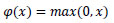
3. The rectified Linear Unit layer (ReLu) uses the function max (0, x). In this case, negative standards are filtered from the images and replaced with zero.
4. The fully connected layer is used to multiply the input by the weight matrix value, and then the value is added to the basis vector value. This, in turn, is connected to multiple layers of similar neural networks.
In this research work, Deep Convolutional Neural Network (CNN) models, including VGG16, VGG19, ResNet 18, ResNet 50, and EfficientNet, are used to address the challenges of real-time polyp recognition. The end-to-end DenseNet models, in which each layer is connected to every preceding layer in a feed-forward manner, were first introduced in DenseNet.
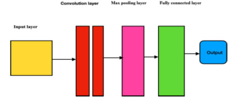
Overview of a convolutional neural network.
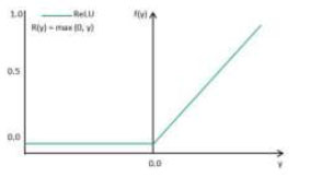
ReLU activation function.
2.1.1. Activation Layer
The addition of the activation layer helps in analyzing the output for a given input. The activation function compares the input value against a threshold, and neurons are activated if the input exceeds this threshold, as illustrated in Fig. (2). ReLU (Rectified Linear Unit) is chosen as the activation function in VGG16, VGG19, ResNet, and EfficientNet models because it helps address a common problem encountered in deep neural networks known as the vanishing gradient problem. The issue arises when gradients become very small as they propagate through multiple layers during training, resulting in slow or stalled learning. By using ReLU, this issue is mitigated as it allows for faster convergence by preventing gradients from becoming too small. Additionally, ReLU introduces sparsity in the network, which encourages the learning of diverse features and improves the model's ability to generalize to unseen data.
ReLU is selected for polyp detection because it helps prevent problems with gradient vanishing, which are important in deep networks. It encourages the model to learn a variety of features, thereby improving its ability to distinguish polyps from healthy tissue. Therefore, using ReLU improves the model's accuracy by making training more efficient and enabling it to represent features effectively in medical images. The mathematical formula is typically inscribed as Equation (1).
| RELU = Max(0,z) | (1) |
Fig. (3) demonstrates the block illustration of the present work. This section provides a detailed description of the methodology being implemented.
2.1.1.1. Input Data
This contains the preprocessed data, which will be passed through the Fastai algorithm. The data contains both polyp and non-polyp data, which have been preprocessed and augmented.
2.1.1.3. Epochs
This term represents the number of times the data must undergo iterations, during which the repetitive training, testing, and validation process occurs.
2.1.1.4. Performance Evaluation
In this part, the analysis of the model is conducted, which is used to monitor and assess how well the model performs at the specific task.
2.1.1.5. Fastai
Fastai is an excellent open-source library developed with the support of PyTorch, aiming to provide better access to AI models and libraries. Its focus on user-friendliness is evident through its high-level API and convenient pre-built functions, which cleverly handle the intricacies of deep learning. With Fastai, users can gain access to various tools for tasks like data preprocessing, model creation, training, and interpretation, all of which are made straightforward.
2.1.1.6. Training Loss
The loss calculated after training the model. It indicates the level of error or inefficiency during training.
2.1.1.7. Validation Loss
The loss calculated using the validation dataset. It reflects the model's inefficiency on unseen data.
2.2. Dataset Details
In this study, two sets of data are employed within the framework of the validation study for polyp recognition. The data sets are sourced from RobFlow, which is an open online platform (https://docs.roboflow.com). The other data sets included are from JSS Hospital for the real-time cross-verification/validation of the model. Table 1 presents the dataset details for each model. In this work, the JSS Hospital data is mixed with the RobFlow dataset. For this purpose, a cleaned dataset and Fastai are used for preprocessing. In this work, 80% of the data is used for testing, 10% of the dataset is used for training, and 10% of the dataset is used for validation.
2.3. DEEP Convolutional Neural Network Models
The following deep learning models are used in Fastai.
• VGG16
• VGG19
• ResNet18
• ResNet50
• EfficientNet
2.3.1. VGG16
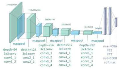
is a pre-trained architecture model that is used in CNN Deep learning work. The model has only 16 layers (16 convolutional layers + 3 max-pooling coats) with trainable weights. It has less reliability with a large number of hyperparameter changes, as shown in Fig. (4). It is considered one of the best vision models developed. The layer names, types, kernel sizes, and filters of the VGG16 model are listed in Table 2.
2.3.2. VGG19
is a pre-trained architecture model that is used in CNN-based deep learning tasks. The model consists of only 19 layers (16 convolutional layers, 5 max-pooling layers, and a softmax layer) with trainable weights. It exhibits less reliability for a large number of hyper-
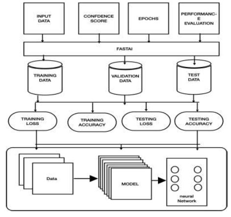
Block Diagram
| Model | Training | Testing | Validation | Total |
|---|---|---|---|---|
| VGG16 | 7800 | 975 | 975 | 9750 |
| VGG19 | 4496 | 562 | 562 | 5620 |
| ResNet50 | 7272 | 909 | 909 | 9090 |
| ResNet18 | 7272 | 909 | 909 | 9090 |
| EfficientNet | 7800 | 975 | 975 | 9750 |
| Block | Layer (name) | Layer (type) | Kernel Size | Filters |
|---|---|---|---|---|
| 1 | CONV 1-1 CONV 1-2 MAX-pooling |
CONVOLUTION CONVOLUTION POOLING | 3*3 3*3 |
64 64 |
| 2 | CONV 2-1 CONV 2-2 MAX-pooling |
CONVOLUTION CONVOLUTION POOLING | 3*3 3*3 - |
128 128 - |
| 3 | CONV 3-1 | CONVOLUTION | 3*3 | 256 |
| CONV 3-2 | CONVOLUTION | 3*3 | 256 | |
| CONV 3-3 | CONVOLUTION | 3*3 | 256 | |
| MAX-pooling | POOLING | - | - | |
| 4 | CONV 4-1 | CONVOLUTION | 3*3 | 512 |
| CONV 4-2 | CONVOLUTION | 3*3 | 512 | |
| CONV 4-3 | CONVOLUTION | 3*3 | 512 | |
| MAX-pooling | POOLING | - | - | |
| 5 | CONV 5-1 | CONVOLUTION | 3*3 | 512 |
| CONV 5-2 | CONVOLUTION | 3*3 | 512 | |
| CONV 5-3 | CONVOLUTION | 3*3 | 512 | |
| MAX-pooling | POOLING | - | - | |
| 6 | FC6 | DENSE | ||
| 7 | FC7 | DENSE |
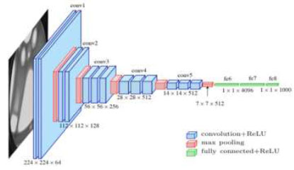
Architecture of the VGG16 model.
parameter changes, as shown in Fig. (5). It is considered one of the best vision models developed. The layer names, types, kernel sizes, and filters of the VGG19 model are listed in Table 3.
2.3.3. VGG Loss
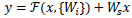
VGG Loss is the Euclidean distance between the feature representation of a reconstructed image GθG (ILR) and the reference image IHR and is given in Equation (2).
 |
(2) |
Where, Wi,j and Hi represent the dimensions with respective feature maps of the VGG network.
Convolution over an image f(x, y) uses a filter w(x, y) that can be calculated using Equation (3). The activation function used in the hidden layers is the rectified linear unit (ReLU) activation function, as given by Equation (4).
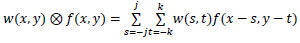 |
(3) |
 |
(4) |
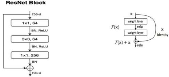
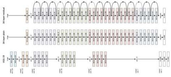
2.3.4. Residual Neural Network
(ResNet18) is a CNN deep learning model used for computer vision applications (Fig. 6). It is a convolutional neural network designed to support hundreds of neural networks; previously, neural networks were limited to a small number of layers. Now, neural networks can have a large number of layers and can be trained for a longer period. ResNet18 is an 18-layer convolution network with 17 convolution layers and a max pooling layer, as shown in Fig. (7).
2.3.5. Residual Neural Network (ResNet50)
ResNet-50 is a convolutional neural network (CNN) design with 50 layers (48 convolutional coats, one max pooling coat, and one normal pooling coat), as shown in Fig. (8). It employs residual connections to ease the training of deep networks and overcome the vanishing gradient problem. ResNet50 is well-suited for computer vision tasks, extracting hierarchical features from input images to achieve good performance in tasks like image classification and object detection.
Convolution is a process that typically reduces the spatial resolution of an image. In the context of residual neural networks, the uniqueness mapping is enhanced by a linear projection W. This multiplication expands the network of the shortcut to contest the residual, which allows the input x and F(x) to be combined as input for the subsequent layers. This combination is given by Equation (5).
 |
(5) |
| Block | Layer (Name) | Layer (Type) | Parameters | Filters |
|---|---|---|---|---|
| 1 | CONV 1-1 CONV 1-2 MAX-pooling |
CONVOLUTION CONVOLUTION POOLING | 1.7K 36K |
64 64 |
| 2 | CONV 2-1 CONV 2-2 MAX-pooling |
CONVOLUTION CONVOLUTION POOLING | 73K 147K |
128 128 - |
| 3 | CONV 3-1 | CONVOLUTION | 300k | 256 |
| CONV 3-2 | CONVOLUTION | 600k | 256 | |
| CONV 3-3 | CONVOLUTION | 600k | 256 | |
| CONV 3-4 | POOLING | 600k | 256 | |
| MAX-pooling | - | |||
| 4 | CONV 4-1 | CONVOLUTION | 1.1M | 512 |
| CONV 4-2 | CONVOLUTION | 2.3M | 512 | |
| CONV 4-3 | CONVOLUTION | 2.3M | 515 | |
| CONV 4-4 | POOLING | 2.3M | 512 | |
| MAX-pooling | - | |||
| 5 | CONV 5-1 | CONVOLUTION | 2.3M | 512 |
| CONV 5-2 | CONVOLUTION | 2.3M | 512 | |
| CONV 5-3 | CONVOLUTION | 2.3M | 512 | |
| CONV 5-4 | POOLING | 2.3M | 512 | |
| MAX-pooling | - | |||
| 6 | FC6 | DENSE | 103M | - |
| 7 | FC7 | DENSE | 17M | |
| Output | 4M |
Architecture of the VGG19 model
Architecture of the ResNet18 model.
Model ResNet block.
Architecture of the ResNet50 model.
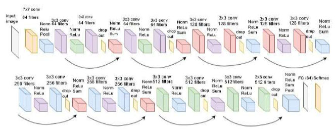
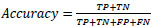
2.3.6. Efficient Net
It is a convolutional neural network construction and scaling technique that consistently scales all proportions of depth/width/resolution using compound coefficients, as shown in Fig. (9). Unlike the normal practice of arbitrarily scaling these factors, the EfficientNet scaling method uniformly scales the network width, depth, and resolution using a set of fixed scaling coefficients (Table 4). Through the output of the neural network, we calculate the overall model's performance. This analysis is conducted using specific equations accordingly. Firstly, we plot a confusion matrix, which provides us with the required parameters as outcomes.
The performance of the CNN network is measured using precision (Equation 6), recall (Equation 7), F1 score (Equation 8), and accuracy (Equation 9), which are computed using the following metrics:
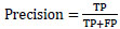 |
(6) |
 |
(7) |
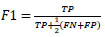 |
(8) |
 |
(9) |
Architecture of the EfficientNet model.
| Stage | Operator | Resolution | Layers |
|---|---|---|---|
| Conv 3*3 | 224*224 | 32 | 1 |
| MB Conv1,k3*3 | 112*112 | 16 | 1 |
| MB Conv6,k3*3 | 112*112 | 24 | 2 |
| MB Conv6,k5*5 | 56*56 | 40 | 2 |
| MB Conv6,k3*3 | 28*28 | 80 | 3 |
| MB Conv6,k5*5 | 14*14 | 112 | 3 |
| MB Conv6,k5*5 | 7*7 | 192 | 4 |
| MB Conv3,k3*3 | 7*7 | 320 | 1 |
| Conv1*1 & Pooling &FC | 7*7 | 1280 | 1 |
3. RESULTS AND DISCUSSION
The analysis involved using various models for image classification, and all of them achieved an impressive accuracy of approximately 99% under different conditions. Both the validation loss and the training loss were comparable, indicating that the models were neither underfitting nor overfitting, striking a good balance.
To demonstrate the results, an interactive website was developed using Hugging Faces and Gradio. This website permits operators to input images and receive real-time forecasts from the trained models. The confusion matrix, which showcases the efficiency of the models in classifying different images, indicates that the classification was nearly perfect.
Overall, the success of the models in achieving high accuracy demonstrates their effectiveness in performing image classification tasks. The website's interactivity
provides an intuitive way for users to witness the models' capabilities in action, making it easy to comprehend their performance. The project's outcome showcases the power of deep learning models in addressing complex image classification challenges with remarkable precision.
3.1. Result of VGG16
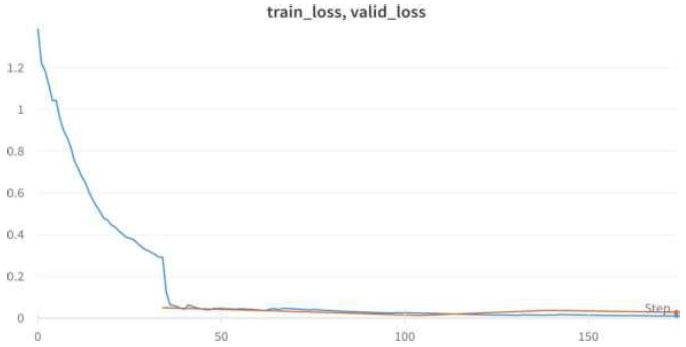
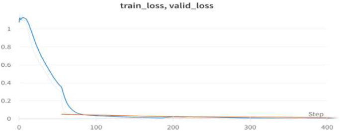
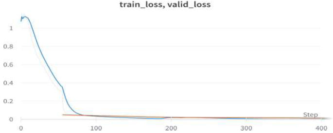
Table 5 shows the epochs loaded. Training loss indicates how well the model fits the training data, while validation loss indicates how well it generalizes to new data. The train/validation loss is shown in Fig. (10), the confusion matrix in Fig. (11), and the image classification of polyps and non-polyps using VGG16 is shown in Fig. (12).
We achieved an accuracy of 99.8% as early as the 4th epoch. The training loss and validation loss for the VGG16 model are shown in Fig. (10).
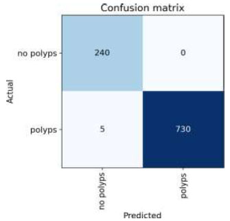
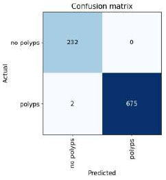
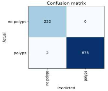
The confusion matrix for the above result is shown in Fig. (11).
The output of the image classification model using Fastai is shown in Fig. (12).
Upon validating the dataset, the VGG16 model displayed promising performance metrics, as shown in Table 6. It achieved an accuracy of 99.48%, indicating that it accurately predicted the outcome for the majority of samples. Moreover, the precision of 100% underscores the model's ability to accurately recognize positive instances among those it labels as positive. In terms of recall, the
| Epoch | Train_loss | Valid_loss | Error_rate | accuracy |
|---|---|---|---|---|
| 0 | 0.093112 | 0.026708 | 0.001026 | 0.998974 |
| 1 | 0.066340 | 0.018183 | 0.001026 | 0.998974 |
| 2 | 0.037638 | 0.015811 | 0.001026 | 0.998974 |
| 3 | 0.029509 | 0.015824 | 0.001026 | 0.998974 |
Train/Valid Loss of VGG16.
Confusion matrix of VGG16.
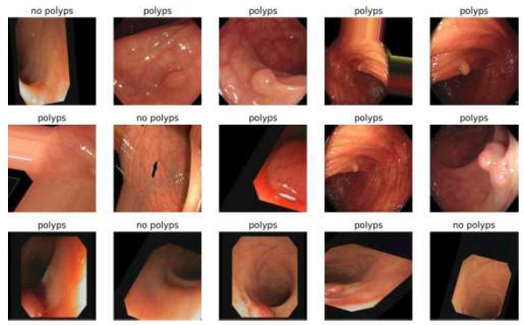
Image Classification of VGG16.
| Metric | Value |
|---|---|
| Accuracy | 0.994872 |
| Precision | 1 |
| Recall | 0.979592 |
| F1 score | 0.989691 |
model successfully captured 97.95% of the actual positive samples in the dataset, demonstrating its effectiveness in identifying relevant cases. Balancing precision and recall, the F1 score stood at 98.96%, affirming the model's overall robustness in handling classification tasks.
3.2. Result of VGG19
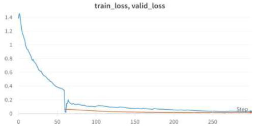
Table 7 shows the epochs loaded. Training loss indicates how well the model fits the training data, while validation loss shows how well the model generalizes to new data. The train/validation loss is shown in Fig. (13), the confusion matrix in Fig. (14), and the image classification of polyps and non-polyps using VGG19 is shown in Fig. (15).
Validation loss and training loss for the above VGG19 model are shown in Fig. (13).
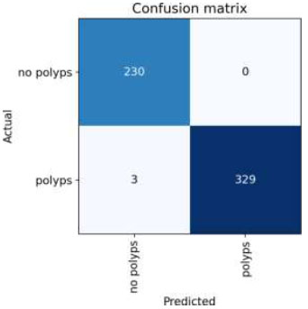
The confusion matrix for the above result is shown in Fig. (14).
The output of the image classification model using Fastai is shown in Fig. (15).
Upon validating the dataset, the VGG19 model also displayed promising performance metrics, as shown in Table 8. It achieved an accuracy of 99.69%, indicating that it accurately predicted the outcome for the majority of samples. Moreover, the precision of 100% underscores the model's ability to accurately identify positive instances among those it labels as positive. In terms of recall, the model managed to capture 98.76% of the actual positive samples in the dataset, demonstrating its effectiveness in recognizing the relevant cases. Balancing precision and recall, the F1 score stood at 98.37%, affirming the model's overall robustness in handling classification tasks.
3.3. Result of ResNet50
Table 9 presents the epochs loaded. The training loss indicates how well the model fits the training data, and the validation loss indicates how well the model fits the new data. The training and validation losses are shown in Figs. (16 and 17). (Fig. 17) illustrates the confusion matrix, and Fig. (18) shows the image classification of polyps and non-polyps using ResNet50.
| Epoch | Train_loss | Valid_loss | Error_rate | Accuracy |
|---|---|---|---|---|
| 0 | 0.291896 | 0.049745 | 0.012456 | 0.987544 |
| Epoch | Train_loss | Valid_loss | Error_rate | Accuracy |
| 0 | 0.045615 | 0.032361 | 0.007117 | 0.992883 |
| 1 | 0.023675 | 0.012731 | 0.007117 | 0.992883 |
| 2 | 0.023675 | 0.012731 | 0.007117 | 0.992883 |
| 3 | 0.015191 | 0.036830 | 0.005338 | 0.994662 |
| Metric | Value |
|---|---|
| Accuracy | 0.996917 |
| Precision | 1 |
| Recall | 0.987654 |
| F1 score | 0.993789 |
Train/valid loss of VGG19.
Confusion Matrix of VGG19.
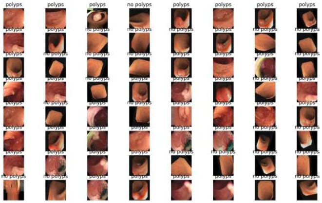
Image classification of VGG19.
| Epoch | Train_loss | Valid_loss | Error_rate | Accuracy |
|---|---|---|---|---|
| 0 | 0.350024 | 0.072139 | 0.011282 | 0.988718 |
| Epoch | Train_loss | Valid_loss | Error_rate | Accuracy |
| 0 | 0.058512 | 0.039168 | 0.007179 | 0.992821 |
| 1 | 0.033305 | 0.025222 | 0.004103 | 0.995897 |
| 2 | 0.014829 | 0.039216 | 0.005128 | 0.994872 |
| 3 | 0.008637 | 0.037751 | 0.005128 | 0.994872 |
We achieved an accuracy of 99.4% as early as the 4th epoch. The training loss and validation loss for the ResNet50 model are shown in Fig. (16).
The confusion matrix for the above result is shown in Fig. (17).
The output of the image classification model using Fastai is shown in Fig. (18).
Upon validating the dataset, the ResNet50 model also displayed promising performance metrics, as shown in Table 10. It achieved an accuracy of 99.79%, indicating that it accurately predicted the outcome for the majority of samples. Moreover, the precision of 100% underscores the model's ability to correctly identify positive instances among those labeled as positive. In terms of recall, the model managed to capture 99.17% of the actual positive samples in the dataset, demonstrating its effectiveness in recognizing the relevant cases. Balancing precision and recall, the F1 score stood at 99.58%, affirming the model's overall robustness in handling classification tasks.
3.4. Result of ResNet18
Table 11 shows the epochs loaded. Training loss indicates how well the model fits the training data, while validation loss shows how well it generalizes to new data. The train/validation loss is shown in Fig. (19), the confusion matrix in Fig. (20), and the image classification of polyps and non-polyps using ResNet18 is shown in Fig. (21).
Train/valid loss of ResNet50.
Confusion matrix of ResNet50.
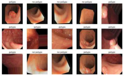
Image classification of ResNet50.
| Metric | Value |
|---|---|
| Accuracy | 0.997942 |
| Precision | 1 |
| recall | 0.991736 |
| F1 score | 0.995851 |
| Epoch | Train_loss | Valid_loss | Error_rate | Accuracy |
|---|---|---|---|---|
| 0 | 0.214846 | 0.040005 | 0.007117 | 0.992883 |
| Epoch | Train_loss | Valid_loss | Error_rate | Accuracy |
| 0 | 0.019264 | 0.142357 | 0.035587 | 0.964413 |
| 1 | 0.018980 | 0.017312 | 0.007117 | 0.994413 |
| 2 | 0.010788 | 0.024240 | 0.003559 | 0.996441 |
| 3 | 0.006357 | 0.023167 | 0.003559 | 0.996441 |
Train/valid loss of ResNet18.
Confusion matrix of ResNet18.
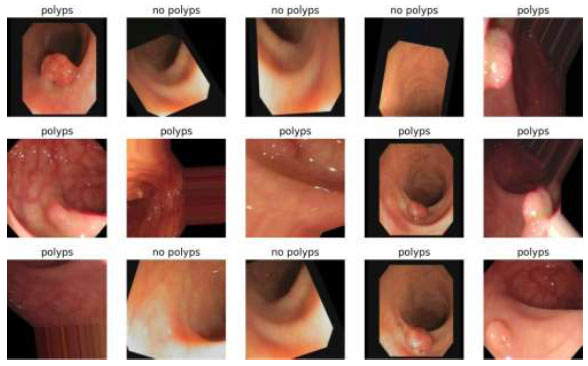
Image classification of ResNet18.
We achieved an accuracy of 99.6% as early as the 4th epoch. The training loss and validation loss for the ResNet18 model are shown in Fig. (19).
The confusion matrix for the above result is shown in Fig. (20).
The output of the image classification model using Fastai is shown in Fig. (21).
Upon validating the dataset, the ResNet18 model displayed promising performance metrics, as shown in Table 12. It achieved an accuracy of 99.79%, indicating that it accurately predicted the outcome for the majority of samples. Moreover, the precision of 100% underscores the model's ability to appropriately recognize positive instances among those it labeled as positive. In terms of recall, the model managed to capture 99.17% of the actual positive samples in the dataset, demonstrating its effectiveness in recognizing the relevant cases. Balancing precision and recall, the F1 score stood at 99.58%, affirming the model's overall robustness in handling classification tasks.
3.5. EfficientNet
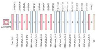
Table 13 shows the epochs loaded. Training loss indicates how well the model fits the training data, while validation loss shows how well it generalizes to new data. The train/validation loss is shown in Fig. (22), the confusion matrix in Fig. (23), and the image classification of polyps and non-polyps using EfficientNet is presented in Fig. (24).
We achieved an accuracy of 99.6% as early as the 4th epoch. The validation loss and training loss for the above EfficientNet model are shown in Fig. (22).
The confusion matrix for the above result is shown in Fig. (23).
The output of the image classification model using Fastai is presented in Fig. (24).
Upon validating the dataset, the EfficientNet model displayed promising performance metrics, as shown in Table 14. It achieved an accuracy of 99.89%, indicating that it accurately predicted the outcome for the majority of samples. Moreover, the precision of 100% underscores the model's ability to correctly identify positive instances among those labeled as positive. In terms of recall, the model managed to capture 99.58% of the actual positive samples in the dataset, demonstrating its effectiveness in recognizing the relevant cases. Balancing precision and recall, the F1 score stood at 99.79%, affirming the model's overall robustness in handling classification tasks. Finally, we can conclude the results by comparing the above results and plotting the graphs of all the models. The training loss and training/validation loss of all the models are shown in Figs. (25 and 26), respectively.
The comparative accuracy plots of the proposed models are given in Fig. (27). From this, the accuracies of VGG16, VGG19, ResNet18, ResNet50, and EfficientNet are 99.89%, 99.46%, 99.48, 99.64%, and 99.64%. From the above results, we can conclude that VGG16 has the best accuracy.
| Metric | Value |
|---|---|
| Accuracy | 0.997942 |
| Precision | 1 |
| recall | 0.991736 |
| F1 score | 0.995851 |
| Epoch | Train_loss | Valid_loss | Error_rate | Accuracy |
|---|---|---|---|---|
| 0 | 0.328127 | 0.042765 | 0.010676 | 0.989324 |
| Epoch | Train_loss | Valid_loss | Error_rate | Accuracy |
| 0 | 0.063772 | 0.19374 | 0.003559 | 0.996441 |
| 1 | 0.032788 | 0.008242 | 0.003559 | 0.996441 |
| 2 | 0.018444 | 0.015641 | 0.003559 | 0.996441 |
| 3 | 0.011566 | 0.011150 | 0.003559 | 0.996441 |
Train/valid loss of EfficientNet .

Confusion matrix of EfficientNet.
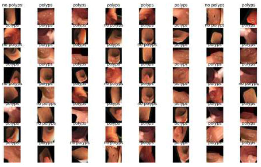
Image classification of EfficientNet.
| Metric | Value |
|---|---|
| Accuracy | 0.99897 |
| Precision | 1 |
| Recall | 0.995851 |
| F1 score | 0.997921 |
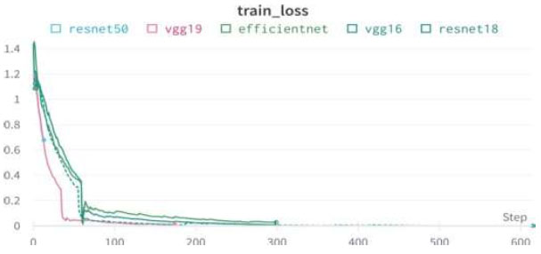
Training loss of all models.
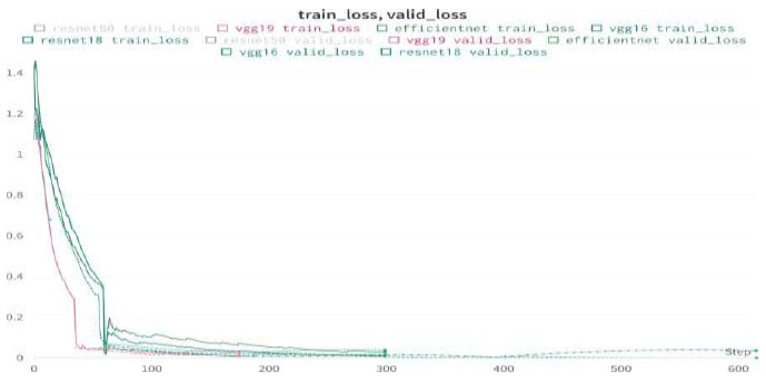
Train/valid loss of all models.
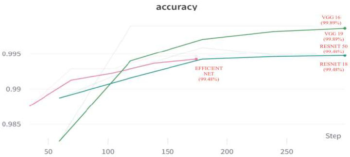
Accuracy of all models.
CONCLUSION
This work investigated various deep CNN learning models, analyzing their functionalities and comparing their performance. After rigorous evaluation, we identified the most efficient models, which were then subjected to a detailed examination of their accuracy, confusion matrices, and probability predictions for all possible scenarios. To ensure the robustness of our findings, we utilized a substantial dataset of around 10,000 samples, allowing us to train our models comprehensively. To make our models easily accessible and user-friendly, we developed a web-based platform using Hugging Face and Gradio libraries. This platform empowers users to predict outcome probabilities simply by uploading an image. Its interactive nature makes it highly practical for a wide range of users. Our efforts culminated in remarkable results, as our models achieved an impressive 99% accuracy in their predictions. Notably, we carefully monitored the risk of overfitting throughout our study and found that our models demonstrated no signs of overfitting. The trial loss and validation loss remained consistently aligned, indicating the generalisability and reliability of our models.
We have successfully leveraged cutting-edge technologies, meticulous model selection, and comprehensive evaluations to deliver a powerful predictive tool. Its potential impact and usability hold great promise for practical applications in various domains.
LIST OF ABBREVIATIONS
| CRC | = Colorectal Cancer |
| CNN - | = Convolutional Neural Network |
| ADR | = Adenoma Detection Rate |
| PDR | = Polyp Detection Rate |
| CTC | = Computed Tomographic Colonography |
| RCTs | = Randomized Controlled Trials |
| MFMC | = Markov Factorization Monte Carlo |
| MCMC | = Markov Chain Monte Carlo |
| NAFLD | = Non-Alcoholic Fatty Liver Disease |
| HCC | = Hepatocellular Carcinoma |
| GWAS | = Genome-Wide Association Study |
| MMR | = Mismatch Repair |
| PDR | = Polyp Detection Rate |
| MSI | = Microsatellite Instability |
| AIC | = AI-Assisted Colonoscopy |
| AMR | = Adenoma Miss Rates |
| CAC | = Computer-Aided Colonoscopy |
| EPAGE | = European Panel On The Appropriateness Of Gastrointestinal Endoscopy |
| ReLU | = Rectified Linear Unit |
| VGG | = Visual Geometry Group |
| ResNet | = Residual Neural Network |
AUTHORS’ CONTRIBUTIONS
Shashidhar R, Suveer Udayashankara, Aradya H V, Vinod Kumar L, and Vikram Patil conceived and designed the study. Shashidhar R, Suveer Udayashankara, Aradya H V, Vinod Kumar L, and Vikram Patil collected the data. Shashidhar R, Suveer Udayashankara, Vinayakumar Ravi, Aradya H V, Vinod Kumar L, and Vikram Patil analyzed and interpreted the results. Shashidhar R, Suveer Udayashankara, and Aradya H V drafted the manuscript. Shashidhar R and Vinayakumar Ravi corrected the manuscript. Shashidhar R and Suveer Udayashankara developed the software. All authors reviewed the results and approved the final version of the manuscript.
AVAILABILITY OF DATA AND MATERIALS
All data generated or analyzed during this study are included in this published article.
CONFLICT OF INTEREST
Vinayakumar Ravi is the associate editorial board member of the journal TOBIOIJ.
ACKNOWLEDGEMENTS
Declared none.