Electrocardiogram Fiducial Points Detection and Estimation Methodology for Automatic Diagnose
Abstract
Background:
The estimation of fiducial points is specially important in the analysis and automatic diagnose of Electrocardiographic (ECG) signals.
Objective:
A new algorithm which could be easily implemented is presented to accomplish this task.
Methods:
Its methodology is rather simple, and starts from some ideas available in the literature combined with new approachs provided by the authors. First, a QRS complex detection algorithm is presented based on the computation of energy maxima in ECG signals which allow the measurement of cardiac frequency (in beats per minute) and the estimation of R peaks temporal positions (in number of samples). From these ones, an estimation of fiducial points Q, S, J, P and T waves onset and offset points are worked out, supported in a simple modified slope method with constraints.
The location process of fiducial points is assisted with the help of the so called curvature filters, which allow to improve the accuracy in this task.
Results:
The procedure is simulated in Matlab and GNU Octave by using test signals from the MIT medical database, Cardiosim II equipment patterns and synthetic signals developed by the authors.
Conclusion:
One of the novelties of this work is the global strategy. Also, another significant innovation is the introduction of the curvature filters. We think this concept will prove to be a useful tool in signal processing, not only in ECG analysis.
1. INTRODUCTION
Electrocardiographic signals (ECG) are a main tool in Medicine, since ECG analysis is a routinary part of any complete medical evaluation. This is due to the fundamental role the heart plays in human health, and because ECG provides a noni nvasive and relatively easy way of knowing how the heart is working [1-8].
Furthermore, recently ECG and EEG (electroencephalographic) signals have proven to be an appropriate tool in fields as security, privacy, communication networks or psychology, in which biometric methods play a role [9-16].
In this context, the estimation of fiducial points of ECG signals is basic for feature extraction, and subsequently, to ECG interpretation. Thus, algorithms and techniques which could accomplish accurately this task are especially important in designing automatic analysis and diagnose tools.
A lot of such methodologies have been developed in the recent decades, which constitutes an active area of research, with multiple challenges still to overcome [1-4, 17-69]. The current work is a contribution to this goal.
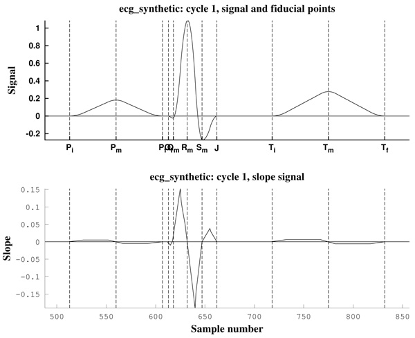
Before to expose our method, let us describe the basic features of an ECG. In the Fig. (1) a typical cycle of an ECG with normal sinus rhythm is shown, with the P, Q, R, S and T waves. In this text, the starting and ending points of P and T waves are labeled Pi, Pf, Ti, and Tf, and its maximum/minimum as Pm and Tm, respectively. The starting point of the QRS complex is labeled Qi, and the ending point J, as is known as the J point. Also, the maximum/minimum of the Q, R and S waves are labeled Qm, Rm and Sm, respectively. Note that, because of its inherent complexity, there are no rigorous definitions of these concepts.
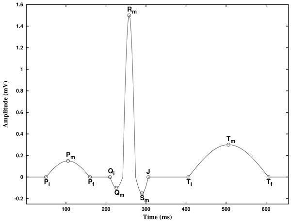
In addition, the piece of the signal between two consecutive Rm points is known as RR interval. Furthermore, the piece of the signal between Pi and the following Qi point is known as PQ (or PR) interval, and the piece of the signal between Qi and the following Tf point is known as QT interval. Analogously, the piece of the signal between the J point and the following Ti point is known as ST segment, and the piece of the signal between Pf and the following Qi point is known as PQ segment [2].
The Table 1 shows the normal values of the main ECG features of a typical lead II in sinus rhythm at a heart rate of 60 bpm for a healthy male adult [2, 23, 70]. We will use these values for testing our methodology by simulating it in practical examples.
| Feature | Normal Value | Normal Limit |
|---|---|---|
| P width (Pf - Pi) | 110ms | +20ms |
| PQ/PR interval (Qi - Pi) | 160ms | +40ms |
| QRS width (J - Qi) | 100ms | +20ms |
| QT interval (Tf - Qi) | 400ms | +40ms |
| ST segment (Ti - J) | 150ms | - |
| T width (Tf - Ti) | 150ms | - |
| P amplitude | 0.15mV | +0.05mV |
| QRS height | 1.50mV | +0.50mV |
| ST level | 0.00mV | +0.10mV |
| T amplitude | 0.30mV | +0.20mV |
In the clinical evaluation of an ECG, physicians currently focus on the following main features [71, 72]:
1.1 Measurement of Cardiac Frequency: It consists on measuring the number of cycles or heartbeats per minute.
1.2 Heart Rate Analysis: The cardiac frequency should be almost constant in a sinus rhythm, when the sinoatrial node acts as the natural pacemaker. In the ECG, this is basically characterized by the fact that each QRS complex is preceded by a P wave.
1.3 Measurement of PR Interval: The PR interval measures the required time for the electrical impulse to traveling from the sinoatrial node to the ventricles. In a health individual, its length is between 120 ms and 200 ms. It is useful to evaluate the signal conduction in the atriums and it could help to identify atrial blocks.
1.4 Heart Vector Estimation: It is computed from I and III (or I and aVF) leads, and it gives information about blocks and hypertrophies.
1.5 Measurement of QT Interval: It gives information about depolarization and repolarization processes of ventricles, and it is related to some abnormalities known as QT syndrome.
1.6 Width of QRS Complex: It represents the time in which ventricles depolarizate, and it is estimated between 80 ms and 120 ms. It is useful to evaluate troubles in the conduction system, as blocks.
1.7 ST Segment: Its width is measured, as well as possible elevation or depression. It is related to ischemic processes, infarcts and other special diseases, as the Brugada syndrome.
8. Special Features of P, Q, R, S and T Waves: Some morphologies are connected to different pathologies.
Note that the diagnose of ECG signals is out of the scope of the current work, so the previous comments are merely orientative. Here we present a methodology for ECG analysis, focusing in the above 1, 2, 3, 5, 6 and 7 points.
2. MATERIALS AND METHODS
2.1. Curvature Filters
Before to proceed to explain the proposed method for ECG analysis, we introduce a new tool for signal analysis (to the best of our knowledge), which we call “curvature filters”. We start by explaining the underlying idea.
The onset and offset of ECG waves are characterized by a noticeable change in the slope of the signal at these points. Usually R waves climb up or fall dramatically, what weakens the influence of noise and makes easier the work of locating them. However, in general these twists are not always easy to find, mainly because of the presence of noise. It is worth to note that noise makes an appropriate slope measurement greatly difficult.
The onset and offset of the P and T waves (here denotated Pi, Pf, Ti and Tf, respectively), as well as the onset of the Q wave (called Qi) and the offset of the S wave, i.e., the J point, sometimes are hard to be found. Frequently, the amplitude of the P wave (or even the T wave) is scarcely greater than the noise intensity. Often, this is also the case of Q and S waves, worsened by the fact of their much more short width. On the other hand, the T wave (and also the other waves) could be preceded or followed by ascending/descending periods of non vanishing slope, thus not completely isoelectric. These preceding periods are not quite different from the proper ascending/descending sides of the T wave. All these circumstances could collude in making these fiducial points almost indistinguishable from regular noise.
In order to be able to catch these twists, and taking into account the previously observed difficulty of measuring slopes under noise, we propose a technique to estimate “local curvature” of the signal.
In order to achieve this goal, we proceed as follows. We look for local information, but we have to average in order to avoid noise effects. On the other hand, the twists or slope changes we are looking for are linked in some sense to the second derivative, in “Calculus language”. Thinking about Taylor approximations, this is nothing but approximate locally a function with second order polynomials. This way of thinking is merely motivational, since we are dealing with discrete signals. Nevertheless, we have found it useful in our simulations. Anyway, consequently, we have to discretize our approximations.
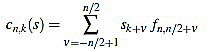
Fix a non negative integer n ≥ 3, which will play the role of the window width. The set of integers will be denoted by  , and the set of real numbers will be denoted by
  . We consider the basic quadratic polynomial p(x) = 3x2 on the interval [- n, n] (the factor 3 is suitable for notation only), and we discretize it by averaging on uniform intervals of length two: For each integer k with 1 ≤ k ≤ n we compute:
 |
(1) |
Thus, we define
 |
(2) |
In order to make the curvature filter orthogonal to constant signals, we subtract the mean
 |
(3) |
Thus, we define for k with 1 ≤ k ≤ n
 |
(4) |
We also set  . Now we get
  from the above computations. One can also check that
 |
(5) |
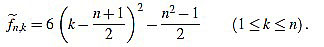
Note that  is integer for k=1,...,n. For the sake of simplicity, the n-th curvature filter is defined by
 |
(6) |
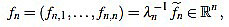
Where the positive integer factor λn is chosen such that the set of integers  is mutually prime (the only positive integer that divides both of them is one). That reduces the size of the filter entries, and does not impact on their use, since any multiple of the curvature filter is equally useful as long as only one order n is used to measure local curvature.
It turns out that the sequence of scaling factors  is easily computed:
Proposition 2.1 The scaling factors in the definition of curvature filters (6) are given by
 |
(7) |
for any m,  such that 0 ≤ p ≤ 12 and n = 12m + p ≥ 3.
We postpone its proof until Appendix A, in order to avoid a disruption in the explanation. Explicit expressions for the curvature filters can be found into this proof, and examples of the first curvature filters can be found listed in Table 2 at Appendix B.
| n | 3 | 4 | 5 | 6 | 7 | 8 | 9 | 10 | 11 | 12 | 13 | 14 | 15 | 16 | 17 | 18 | 19 | 20 | 21 | 22 | 23 | 24 | 25 |
| || fn ||2 | 6 | 4 | 14 | 84 | 84 | 168 | 2772 | 132 | 858 | 12012 | 2002 | 728 | 37128 | 5712 | 7752 | 23256 | 13566 | 17556 | 201894 | 7084 | 35420 | 394680 | 53820 |
| 1 2 3 4 5 |
1 -2 1 - - |
1 -1 -1 1 - |
2 -1 -2 -1 2 |
5 -1 -4 -4 -1 |
5 0 -3 -4 -3 |
7 1 -3 -5 -5 |
28 7 -8 -17 -20 |
6 2 -1 -3 -4 |
15 6 -1 -6 -9 |
55 25 1 -5 -10 |
22 11 2 -5 -10 |
13 7 2 -2 -5 |
91 52 19 -8 -29 |
35 21 9 -1 -9 |
40 25 12 1 -8 |
68 44 23 5 10 |
51 34 19 6 -5 |
57 39 23 9 -3 |
190 133 82 37 -2 |
35 25 16 8 1 |
77 56 37 20 5 |
253 187 127 73 25 |
92 69 48 29 12 |
| 6 7 8 9 10 |
- - - - - |
- - - - - |
- - - - - |
5 - - - - |
0 5 - - - |
-3 1 7 - - |
-17 -8 7 28 - |
-4 -3 -1 2 6 |
-10 -9 -6 -1 6 |
-35 -35 -29 -17 1 |
-13 -14 -13 -10 -5 |
-7 -8 -8 -7 -5 |
-44 -53 -56 -53 -44 |
-15 -19 -21 -21 -19 |
-15 -20 -23 -24 -23 |
-22 -31 -37 -40 -40 |
-14 -21 -26 -29 -30 |
-13 -21 -27 -31 -33 |
-35 -62 -83 -98 -107 |
-5 -10 -14 -17 -19 |
-8 -19 -28 -35 -40 |
-17 -53 -83 -107 -125 |
-3 -16 -27 -36 -43 |
| 11 12 13 14 15 |
- - - - - |
- - - - - |
- - - - - |
- - - - - |
- - - - - |
- - - - - |
- - - - - |
- - - - - |
15 - - - - |
25 55 - - - |
2 11 22 - - |
-2 2 7 13 - |
-29 -8 19 52 91 |
-15 -9 -1 9 21 |
-20 -15 -8 1 12 |
-37 -31 -22 -10 5 |
-29 -26 -21 -14 -5 |
-33 -31 -27 -21 -13 |
-110 -107 -98 -83 -62 |
-20 -20 -19 -17 -14 |
-43 -44 -43 -40 -35 |
-137 -143 -143 -137 -125 |
-48 -51 -52 -51 -48 |
| 16 17 18 19 20 |
- - - - - |
- - - - - |
- - - - - |
- - - - - |
- - - - - |
- - - - - |
- - - - - |
- - - - - |
- - - - - |
- - - - - |
- - - - - |
- - - - - |
- - - - - |
35 - - - - |
25 40 - - - |
23 44 68 - - |
6 19 34 51 - |
-3 9 23 39 57 |
-35 -2 37 82 133 |
-10 -5 1 8 16 |
-28 -19 -8 5 20 |
-107 -83 -53 -17 25 |
-43 -36 -27 -16 -3 |
| 21 22 23 24 25 |
- - - - - |
- - - - - |
- - - - - |
- - - - - |
- - - - - |
- - - - - |
- - - - - |
- - - - - |
- - - - - |
- - - - - |
- - - - - |
- - - - - |
- - - - - |
- - - - - |
- - - - - |
- - - - - |
- - - - - |
- - - - - |
190 - - - - |
25 35 - - - |
37 56 77 - - |
73 127 187 253 - |
12 29 48 69 92 |
 , and the filter entries fn,k (for k = 1,...,n).
In virtue of identity (5) the filter entries are symmetric with respect to (n+1)/2. Consequently, the curvature filter is also orthogonal to linear signals. It is worth to note that symmetry implies that only the half of filter entries fn,k need to be computed.
Given a signal  its k-th curvature coefficient of order n is
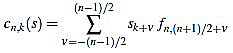 |
(8) |
if n is odd, and
 |
(9) |
if n is even.
Because of the above computations, the curvature filter fn is orthogonal to affine signals: for any  we have
 |
(10) |
That means that the curvature coefficients are insensitive to the signal level and slope. This property is important, since we want the curvature filters for measuring only slope changes, not the slope or the proper signal itself.
If one wants to use only curvature coefficients of the same order, these definitions with integer fn,k are enough. However, if one wants to compare curvature features corresponding to different orders n, an appropriate normalization is convenient.
We define the normalized curvature filter  by
by
 |
(11) |
Given a signal  , for any
  its k-th normalized curvature coefficient of order n is
 |
(12) |
Explicit expressions can be also easily found for the normalized curvature filters:
Theorem 2.2 For any n ≥ 3 the normalized curvature filter entries are given (for 1 ≤ k ≤ n) by
 |
(13) |
These formulae come from (4), (5), and the following result.
Proposition 2.3 For any integer n ≥ 3 one has
 |
(14) |
We postpone its proof until Appendix A, in order to avoid a disruption in the explanation.
2.1.1. Choice of Curvature Filter Orders
In order to obtain an accurate result in using curvature filters for wave onset and offset estimation, an appropriate order n must be chosen on each case. In this section we argue about how to choose this optimal order. In order to do that, we test the curvature filters on a test example designed for offset estimation. The picture for onsets is completely similar because of symmetry.
We fix a time wave length wt, in milliseconds, and a corresponding wave length ws, in number of samples. The estimated sampling frequency is then obtained by the formula Fs ~ 1000ws/wt, in Hertzs, where this quantity is rounded to the closest integer. The base signal is composed by a semi ellipse of length ws samples and height h (in millivolts), followed by ws zeroes. Consequently, the signal length is 2ws. The base signal is perturbed with random noise of a given intensity hn (in millivolts), giving a set of Nt perturbed signals of length 2ws.
In the next test example we use the following values: wt=110 ms, h=0.15 mV, hn=0.01 mV, and Nt=100 signals (according to the P wave in the Table 1). The wave lengths used to test the curvature filters in this example go from ws=3 samples up to ws=100 samples, by increments of 1 sample.
Next, for each noisy signal sj (with j=1,...,Nt), and for each order n (with n=3,...,2ws-1), we compute the corresponding normalized curvature coefficients. Note that we do that only for sample points such that the window is completely included into the signal range, as we are dealing with a finite signal; that depends on the order n of the curvature filter used. Then, we estimate the offset by selecting the greatest normalized curvature coefficient; thus, its offset is defined as the corresponding sample point k=oj,n with greatest normalized curvature coefficient. Note that, as we are looking for offsets for upward waves, we might select points with maximum convexity; i.e., greatest positive curvature.
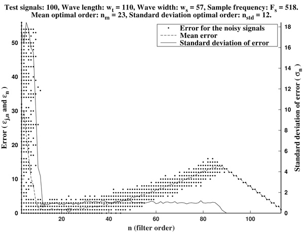
In Figs. (2 and 3) we show the resulting estimated offsets oj,n for j=1,...,Nt, and n=3,...,2ws-1, for the wave lengths ws=15 samples (corresponding to Fs=136 Hz) and ws=55 samples (corresponding to Fs=500 Hz). We consider as a reference correct offset the sample point k=ws.
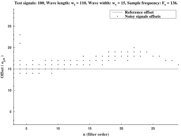
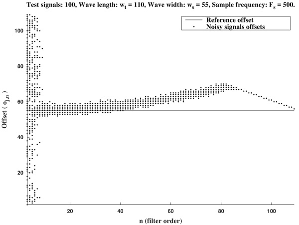
In view of Figs. (2 and 3) and the rest of simulations, several comments arise about the curvature filters performance:
- If the curvature filter order is too small, then the noise has a profound effect in the curvature coefficients. That is, low order curvature filters do not distinguish between signal twists and noise.
- From certain large enough order, curvature filters are very proficient on the task of detecting the offset.
- The accuracy of the measurement slightly deteriorates as the order increases. On average, a trend to shift outwards the wave is detected.
- The latter convergence for very high orders is spurious since is due to the finite character of the signal.
These remarks suggest that curvature filters could be an useful tool on detecting fiducial points in ECG signals, provided that a suitable order is chosen for the specific task. We think this is valid also for features extraction in signal processing, in general.
In order to measure quantitatively the curvature filters performance in the test example, we define the error as  =
=  (ws being fixed), for any j=1,...,Nt, and n=3,...,2ws-1. Thus, for each order n we compute the mean error
 |
(15) |
Then, the mean optimal order is defined as the (smallest) order n=nm for which  is minimum
  . In other words, the mean optimal order is the window size for which the greatest-curvature-coefficient method (i.e., the previous one) for detecting the offset is more accurate, on average. Note we avoid too large orders in this criteria.
Another important features which are also highly desirable, apart from accuracy, are fiability and robustness under noise presence. In order to take into account these aspects, we also analyse the measurements error dispersion provided by the greatest-curvature-coefficient method. Hence, we consider the error standard deviation
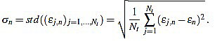 |
(16) |
In Figs. (4 and 5) we see that the magnitude of the errors dramatically falls off after the initial noise-sensitive period, as expected from the above remarks based on Figs. (2 and 3). Coherently, the mean error and the error standard deviation σn also have the same behavior. We define the standard deviation optimal order as the first order n=nstd such that σn ≤ σn+1 and σn is lower than a reference value empirically set to 2. That is, we look for a small enough local minimum of the standard deviation.
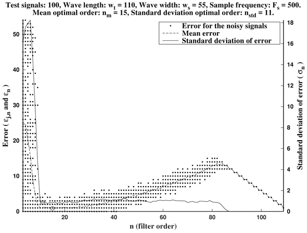
As it has been remarked before, immediately after the initial noise-sensitive period the greatest-curvature-coefficient method performs very well, providing a quite low mean error almost stagnant in a long period on n. The same could be said for the standard deviation of the error.
As it is illustrated in Fig. (6), it often occurs that the mean optimal order unnecessarily increases to larger values. Due to computational reasons, it is preferable to use low order filters as long as possible. Another factor to bear in mind is that, generally, waves do not occur isolated in an ECG, but surrounded by other ones. Hence, too high orders are undesirable since the presence of neighboring waves could cause interference.
In order to avoid that, we recommend as a preferential choice the standard deviation optimal order nstd to be used in the greatest-curvature-coefficient method.
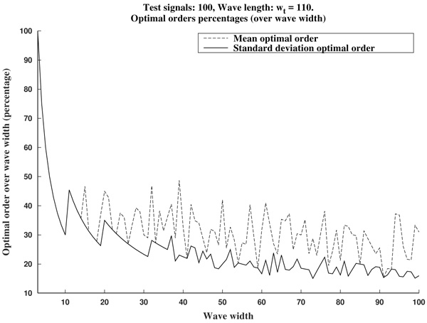
In Fig. (7) we can see the optimal orders (mean optimal order nm and standard deviation optimal order nstd) for ws in the proposed range (that is, wave lengths from ws=3 samples up to ws=100 samples, by increments of 1 sample).
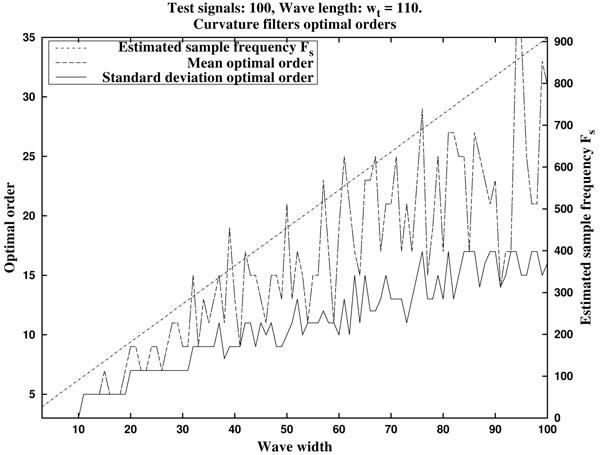
In summary, in view of Fig. (8), we recommend to use a curvature filter order between the 15% and the 30% of the wave width ws. These values should be increased for very low sampling frequencies, as the resulting from Holter monitors. This quantity could be estimated a priori from the estimated wave length wt (in milliseconds, which could be taken from references as in Table 1), and the signal sampling frequency Fs (in Hertz), which is assumed to be known, by the formula.
 |
(17) |
2.2. Description of Methodology
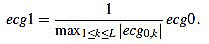
In this section we will describe our proposal of methodology for the analysis and features extraction of ECG signals. Suppose we have a non trivial ECG signal, denoted ecg0, of length L. That is,  is a vector of L real components. We will denote by Fs the sample rate (sampling frequency) with which the ECG signal was taken, measured in Hertzs (Hz).
2.2.1. Preprocessing
Generally, the ECG signal is assumed to be contaminated with several noise sources. This noise could be reduced by using some filters which cut off different frequencies, but definitely cannot be completely avoided. Anyway, for this reason and previous to the feature extraction process, a preprocessing is necessary to be applied to the signal. Consequently, the original signal suffers changes which add some uncertainty to the final results. This phenomena is specially remarkable in the case of P and T waves onset and offset location. That is why we speak about feature “estimation”, and not about “measurement”.
First of all, the amplitude of the original signal is normalized to 1:
 |
(18) |
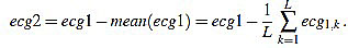
The resulting signal  has amplitude 1. Next, the direct level is supressed, obtaining a signal
  given by
 |
(19) |
Obviously, one has mean (ecg2)=0.
After that, a high pass filter of type Butterworth of order 2 is applied to filter ecg2, with a cut frequency of 0.5 Hz, to obtain a preprocessed signal  . This step is always present in ECG professional applications, in order to remove very low frequencies.
When applying this preprocessing to signals from the MIT database [73], which proceed from Holters, this last step is very important and helps to improve the accuracy in subsequent estimations. On the other hand, when dealing with signals from pattern generating devices, it is usually required an additional filtering of smoothing or averaging type. In general, the required preprocessing highly depends on the measurement system features used to generate the ECG signal, and could include the use of other filters, as interference supressing filters out of 60 Hz. For the signals we have used in this work, this is not the case.
2.2.2. Rm Peaks Location and Heart Rate Analysis
QRS complex detection is considered a fundamental step in the analysis of ECG signals, because of measurement and characterization of different associated parameters rely on the accuracy with which it is performed [2, 19]. On the one hand, from the QRS complex cardiac frequency can be obtained, and subsequently heart rate is also obtained. On the other hand, Rm peaks almost delimitate each heart beat (more clearly than other waves) in such a way that estimation of the other fiducial points is more easily carried out from them.
In the recent decades many QRS complex detection methods have been reported in the literature [1, 2, 4, 17-19, 24], and references therein), including derivatives approximation, digital filters, wavelets, adaptative filters, neural networks, hidden Markov models or mathematical morphology, among other techniques.
In this work, we make use of the techniques developed in the literature [24]. Concretely, we select the pre-processed signal energy maximum, choosing a threshold which is empirically set. An appropriate choice of these maximum allows to obtain the heart rate (in beats per minute). Moreover, we describe two different methods to locate the Rm peaks in the original signal (in number of samples): one can simply extract the maximum peaks, or one can perform a crossed correlation between the filtered signal and the original signal (normalized and prefiltered).
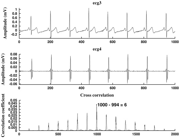
We start with the preprocessed signal ecg3. Previous to energy processes, we filter it by using a band pass filter, in the band 10-25 Hz or 15-20 Hz, obtaining a filtered signal  . This step is mandatory in order to remove artifacts, interferences, and the influence of P and T waves. Note that in this moment we are only interested in detecting Rm peaks (Fig. 9).
Next, we consider the energy signal E4 given by E4 = 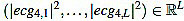 . The energy threshold Eth is empirically set to the value
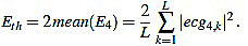 |
(20) |
Then, the energy maximum are extracted with the constraint E4 > Eth. In the MATLAB code, the energy peak extraction is performed by using the implemented built-in function findpeaks [74]. The resulting energy peaks have to be sifted out, since they usually appear pairs of “peaks” which are unnaturally quite close (presumably corresponding to the same R wave, due to the noise and filtering processes). These related peaks have to be removed, since they produce non physiological values for the cardiac frequency.
Each energy peak corresponds to an Rm peak, but the last ones need to be located, since the band pass filtering provokes a constant gap between the two signals, which shifts the peaks in time.
What we do is to compute the cross-correlation and finding the correlation coefficient between the energy E4 of the filtered signal and the energy E3 (given by  ) of the original preprocessed signal. Then, the shift is the difference between the signal length L and the lag corresponding to the correlation coefficient Kcr, the maximum of the cross correlation. In that way, we are able to locate the Rm peaks in the original preprocessed signal ecg3. In the code, the cross-correlation analysis is performed by using the MATLAB built-in function xcorr [74].
Once the Rm peaks of ecg3 are located, the RR intervals are known. The widths of RR intervals, or distance between consecutive Rm peaks, allow to compute the approximated cardiac frequency: If LRR is the width of a given RR interval (in number of samples), and HR is the heart rate (measured in beats per minute bpm), then
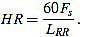 |
(21) |
2.2.3. QRS Complex Location
In order to describe the QRS complex, we have to locate the Qi, Qm, Sm and J points of each cycle. Here, for exposition purposes, we consider the Rm point as the maximum of the R wave, and the Qm and Sm points are understood as the minimum of the Q and S waves, respectively. In addition, Qi is the starting point of the Q wave and the end of the PQ segment, and J is the ending point of the S wave and the start of the ST segment.
For this task, we proceed by using a modified slope analysis method with restrictions, starting from a peak. This algorithm is inspired by Chapter 9 of [2]. The basic idea is to descend/ascend from a maximum/minimum, respectively, until a change in the sign of the slope is found. On a given sample point k (with 1 ≤ k < L), the slope of the signal ecg3 is defined by
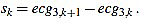 |
(22) |
This method is justified because of in the pronounced ascents and falls of the signal, the influence of the noise is quite lower than in the isolectric segments.
In this analysis we remove the first and final cycles, since they could be incomplete or distorted because of the original signal capture process. Then, consider the original preprocessed signal ecg3, and fix some Rm peak (not the first, not the last one).
On the one hand, we move backward from the Rm peak until we find the first local minimum; that is, until we find a point k whose left neighbor has nonpositive slope sk-1 ≤ 0. This point is defined as the Qm point of this cycle. From this point, we continue backward looking for the first local maximum; that is, a point k such that its left neighbor has nonnegative slope This point is defined as the sk-1 ≥ 0. This point is defined as the Qi point of this cycle.
On the other hand, we proceed analogously to the right. From the Rm peak, we move forward until we find the first local minimum; that is, until we find a point k with nonnegative slope sk ≥ 0. This point is defined as the sm point of this cycle. From this point, we continue forward looking for the first local maximum; that is, a point k with nonpositive slope sk ≤ 0. This point is defined as the J point of this cycle.
In practice, this method needs to be complemented with different criteria about how far the search should go, related to the estimated length of the Q and S waves. This is because of, depending on the presence or absence of Q and S waves in the ECG signal, the pure slope analysis algorithm could produce fiducial points far away from the Rm peak, which would be unnatural. On the other hand, the greatest/smallest-curvature-coefficient method could assist the slope analysis method, as in the following subsection is illustrated, specially in the case of the Qi and J points. However, the short width of these waves forces to use a quite small order, which could be imprecise, specially for signals with very low sampling frequency.
2.2.4. Estimation of Remaining Fiducial Points
At this point, what remains is to estimate the fiducial points in P and T waves. We proceed by using a modified slope analysis method [2], as before, combined with the use of curvature filters.
First of all, we find the Pm and Tm peaks. Without loss of generality, we assume we deal with upward P and T waves. The case of downward waves is completely analogous, and an algorithm to distinguish between upward and downward cases is easy to implement by computing maximum and minimum and comparing them (Qi and J points could be taken as isoelectric reference level for the comparison, respectively).
Hence, from the Rm peak, we look for a global maximum in a preestablished backward/forward range of samples of the signal, respectively. This range could be estimated from the reference values for the PQ and QT intervals (Table 1), the sampling frequency and the previously estimated fiducial points. Thus, the left maximum corresponds to Pm, and the right one corresponds to Tm.
From each one of these points, we descend in order to find the corresponding onset and offset points. The idea is to scan the surrounding signal looking for suitable candidates by using the slope analysis algorithm, and then selecting the best choice with the aid of the curvature filters. The process is as follows.
We start from the Pm point (the process for the T wave is completely analogous). On the one hand, we move backward inside a preestablished range looking for local minimum: Points k whose left neighbors have nonpositive slope sk-1 ≤ 0. At each step, we store them as candidates. When the Range is exhausted, we select the winner by the greatest-curvature-coefficient method: We compute the curvature coefficients of the candidates, and the sample with greatest one among them is designated as the Pi point of the cycle. On the other hand, from the Pm peak we move forward inside a preestablished range (never farther than the corresponding Qi point) looking for local minimum: points k with nonnegative slope sk ≥ 0. They are the candidates, and the Pf is selected among them by the greatest-curvature-coefficient method.
Note that a stopping criteria is necessary in this algorithm. As before, the ranges could be estimated from the reference values for the PQ and QT intervals (Table 1), the sampling frequency and the previously estimated fiducial points. Also, it could happen that candidates which are quite close to the Pm/Tm peaks, respectively, might have to be removed, as at the top of the P and T waves they could exist points with high curvature coefficients, specially in cases of nonstandard morphologies. Consequently, a starting criteria could be also necessary. On the other hand, suitable curvature filters orders for the P and T waves need to be chosen for a well performance of the algorithm (subsection 2.1.1.).
3. RESULTS
Next we show some examples of application of this methodology. For QRS complex detection, the modified slope analysis method was used, aided by range criteria based on estimated wave widths. For P and T waves estimation, a combined slope analysis and curvature filters method was used, aided with an starting/stopping criteria based on estimated wave widths (Table 1). In the simulations presented here, the used curvature filters orders were n=3 for the QRS complex, and n=5 for the P and T waves, in the case of Fs=128 Hz, and n=9,11,13 for the QRS complex, P and T waves, respectively, in the case of Fs=500 Hz (Fig. 7). Odd orders are prefered because of they center the fiducial point in a better way.
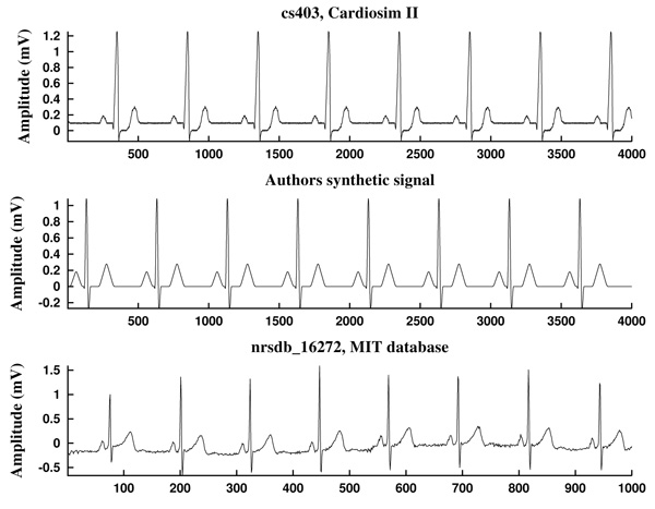
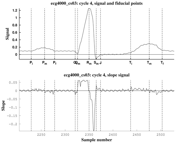
The first ECG signal is cs403, generated by a Cardiosim II device [75] by using the pattern 03, a reference pattern of a normal ECG. The second one is a synthetic ECG signal made by the authors, simulating also a normal sinus rhythm but without noise. Both have a heart rate of HR=60 bpm and a sampling frequency of Fs=500 Hz (Fig. 10).
As can be observed in Fig. (11), the signal slope, defined by (22), gives information about the increase of the ECG signal. However, in Figs. (12) it is clear that noise deeply affects to the signal slope. In that context, curvature filters help to avoid noise in order to find the fiducial points, since they regularize the signal. This effect is due to the fact that the curvature coefficients are weighted averages of the signal.
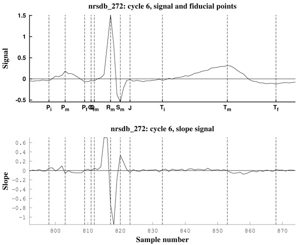
The third example is a piece of 8 cycles of nrsdb_16272, a real ECG signal from the normal sinus rhythm data base from the PhysioBank (MIT database [73]), reported with sampling frequency Fs=128 Hz and nominal HR=60 bpm. In Fig. (13) a cycle of this signal is shown, with estimated fiducial points.
All measurements have been taken with a level of noise, measured in the isoelectric segment which follows the P waveform, between Pf and Qi, lower than 1.33 x 10⁻⁴mV2/Ω (a power of around 100 pW). This is equivalent to a signal contaminated with a maximum random noise of 0.01 mV in amplitude before the operation of prefiltering. That justifies the choice hn at subsection 2.1.1.
From the standpoint of signal to noise ratio S/N, a good performance criterion is obtained with S/N ≥ 20dB, figure of merit kept also in the measurements above [23, 76, 77]. In all cases the power was estimated through the var function of Matlab which gives the signal variance [74].
4. DISCUSSION
Here we have presented a methodology for estimating the fiducial points of an ECG signal. Other features or measurements of interest, as widths of intervals and segments, wave heights, cardiac frequency, heart rate analysis can be computed from the located fiducial points.
One of the novelties of this work is the global strategy: first we localize the R, P and T waves peaks, and then we move backward/forward to the onset/offset, respectively. In this way, we are able to reduce the impact the noise has in the location process.
Also, another significant innovation is the introduction of the curvature filters. We think this concept will prove to be an useful tool in signal processing, not only in ECG analysis.
Moreover, it is worth to note that the combination of the greatest/smallest-curvature-coefficient method and the slope analysis method is significantly more effective than each of them separately: The first one adds accuracy and robustness to the second one, and the last one adds efficiency to the first one, as it reduces much more the number of curvature coefficients to be computed. Note that the signal slope is computationally cheaper than curvature coefficients.
It is worth to note that our method is specially designed to be applied to ECG signals corresponding to a normal sinus rhythm. However, we expect that the philosophy under the method, and specifically the curvature filters as a tool, will be useful in analyzing ECG signals corresponding to heart disorders which can significantly change the rhythm of the heart beat.
CONCLUSION
In the present work we propose a methodology for estimating the fiducial points of an ECG signal, partly based on an introduced tool for signal processing, the curvature filters. This task is expected to be continued in subsequent works. Concretely, one of our main research lines is continue to exploting the curvature filters and related tools potential for ECG analysis.
ETHICS APPROVAL AND CONSENT TO PARTICIPATE
Not applicable.
HUMAN AND ANIMAL RIGHTS
No Animals/Humans were used for studies that are base of this research.
CONSENT FOR PUBLICATION
Not applicable.
CONFLICT OF INTEREST
The authors declare no conflict of interest, financial or otherwise.
ACKNOWLEDGEMENTS
Authors acknowledge Benemérita Universidad Autónoma de Puebla-VIEP financial support through project 00438 “Captura y procesamiento de señales bioeléctricas” granted to AFC, call 2017, and also CONACYT financial support of MSB through “Cátedras CONACYT para Jóvenes Investigadores 2016” program.
The authors thankfully acknowledge the computer resources, technical expertise and support provided by the Laboratorio Nacional de Supercómputo del Sureste de México, CONACYT Network of National Laboratories.
Authors acknowledge the anonymous referees their useful comments and suggestions which have been improved this text.
Authors contributions are as follows: Dr. Yáñez performed the software design and computational simulations. Dr. Soto performed the theoretical analysis and assisted with the software design. Dr. Fraguela designed the research line and performed the theoretical analysis.
APPENDIX A
Proofs
In this section we provide proofs for Proposition 2.1 and Proposition 2.3.
Proof of Proposition 2.1: we recall that the values for the scaling factors in the definition of curvature filters (6) are provided in (7). The argument is a combination of ideas from Elementary Arithmetic, and goes as follows: for any p, from equation (4) we obtain an expression for f12m+p,k by factorizing 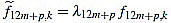 for k=1,...,12m+p, and we make sure that
 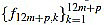 are integers.
Next, we prove that they are mutually prime. If some integer is a common divisor of the filter entries, then has to divide any difference of them. Particularly we compute the difference of two consecutive central entries, around the index value (n+1)/2, because of they are the mutually closest ones. By using this fact we reduce the list of candidates so much. From this, it is straightforward to check there is no common divisors different from +1 or -1.
Details are shown up next for every case:
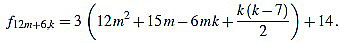
● p=0: we have λ12m = 2 and for k=1,...,12m
 |
(23) |
Since f12m,6m+2-f12m,6m+1 = 6, the common divisors divide 6. But 2 nor 3 divide no f12m,k. Note that k(k-1) is even for any integer k.
● p+1: we have λ12m+1 = 6 and for k=1,...,12m+1
 |
(24) |
Since f12m+1,6m+2-f12m+1,6m+1 = 3, the common divisors divide 3. If 3 divides m, then it is easily seen that 3 does not divide f12m+1,2, and if 3 does not divide m, one can easily check that 3 does not divide f12m+1,1.
● p=2: we have λ12m+2 = 12 and for k=1,...,12m+2
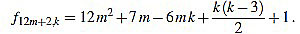 |
(25) |
Note that k(k-3) is even for any integer k. Since f12m+2,6m-f12m+2,6m+1 = 1, we have finished.
● p=3: we have λ12m+3 = 2 and for k=1,...,12m+3
 |
(26) |
Since f12m+3,6m+1-f12m+3,6m+2 = 3, the common divisors divide 3, but 3 divide no f12m+3,k.
● p=4: we have λ12m+4 = 6 and for k=1,...,12m+4
 |
(27) |
Since f12m+4,6m+1-f12m+4,6m+2 = 1, we have finished.
● p=5: we have λ12m+5 = 6 and for k=1,...,12m+5
 |
(28) |
Since f12m+5,6m+2-f12m+5,6m+3 = 1, we have finished.
● p=6: we have λ12m+6 = 4 and for k=1,...,12m+6
 |
(29) |
Since f12m+6,6m+2-f12m+6,6m+3 = 3, the common divisors divide 3, but 3 divide no f12m+6,k. Note that k(k-7) is even for any integer k.
● p=7: we have λ12m+7 = 6 and for k=1,...,12m+7
 |
(30) |
Since f12m+7,6m+3-f12m+7,6m+4 = 1, we have finished.
● p=8: we have λ12m+8 = 6 and for k=1,...,12m+8
 |
(31) |
Since f12m+8,6m+3-f12m+8,6m+4 = 2, the common divisors divide 2, but f12m+8,2 is odd.
● p=9: we have λ12m+9 = 2 and for k=1,...,12m+9
 |
(32) |
Since f12m+9,6m+4-f12m+9,6m+5 = 3, the common divisors divide 3, but 3 divide no f12m+9,k.
● p=10: we have λ12m+10 = 12 and for k=1,...,12m+10
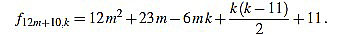 |
(33) |
Note that k(k-11) is even for any integer k. Since f12m+10,6m+4-f12m+10,6m+5 = 1, we have finished.
● p=11: we have λ12m+11 = 6 and for k=1,...,12m+11
 |
(34) |
Since f12m+11,6m+5-f12m+11,6m+6 = 1, we have finished.
Proof of Proposition 2.3: from (5) we have
 |
(35) |
 |
(36) |
Now we compute these two sums separately. On the one hand,
 |
(37) |
In order to compute the other sum, we split in two cases. We will make use of the well known Faulhaber formulas: for any positive integer N, one has
 |
(38) |
 |
(39) |
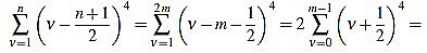
If n is odd, then there exists a positive integer m such that n=2m-1. Then
 |
(40) |
 |
(41) |
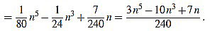
On the other hand, if n is even, then there exists a positive integer m such that n=2m. Then
 |
(42) |
 |
(43) |
 |
(44) |
Note that in both cases we obtain the same expression.
Finally, we have
 |
(45) |
 |
(46) |