A Numerical Investigation of Anatomic Anterior Cruciate Ligament Reconstruction
Abstract
Introduction:
Anterior Cruciate Ligament (ACL) reconstruction by anatomic method is the most popular method of reconstruction. This method of ACL reconstruction utilizes Anteromedial Portal (AMP) techniques.
Methods:
In this study, five human subjects with healthy knee joints were considered on which Lachman test was simulated. Traditional Transtibial (TT) and AMP techniques were simulated in this study. The mean value of Von – Mises stress on the ACL was calculated. ACL reconstruction using hamstring tendon graft was simulated in a finite element analysis on four healthy human knee joints. Magnetic Resonance Images (MRI) of knee joints of four healthy human subjects were analyzed in this study for statistical significance of the results. Both techniques were simulated in each of the subjects. The hamstring tendon graft used had a diameter of 9 mm. The tibial foot print was 44.6 ± 2.5% from the anterior margin and 48 ± 3% from the medial margin. The femoral foot print was calculated based on Mochizuki’s method at 38.7 ± 2.7% from the deep subchondral margin.
Results:
The obliquity of reconstructed – ACL (R – ACL) to the tibial plateau for AM technique was in the range of 51 to 58 degrees in the sagittal plane and 69 to 76 degrees in the coronal plane. In the case of TT technique, it was in the range of 59 to 69 degrees in the coronal plane and 72 to 78 degrees in the coronal plane in the femur. Similarly, the sagittal obliquity of R – ACL in the tibia was 55 degrees. The mean Von–Mises stress in the R – ACL for AMP technique was 17.74 ± 3.01 MPa. The stresses in the R – ACL for AMP technique is consistently near to the mean stress in the intact ACL. Whereas, stresses in the R – ACL used in TT technique are not consistently near to the stresses in the intact ACL of a healthy human knee joint.
Conclusion:
Hence, AMP technique is the better technique between AMP and TT techniques of ACL reconstruction.
1. INTRODUCTION
Human knee joint comprises of femur, tibia and fibular bones. Its main stabilizing ligaments are Anterior Cruciate Ligament (ACL), Posterior Cruciate Ligament (PCL), Lateral Collateral Ligament (LCL) and Medial Collateral Ligament (MCL). The anterior – posterior motion is primarily stabilized by ACL and PCL, while lateral–medial motion is stabilized by LCL and MCL. Most of the human knee joint injuries relate to the rupture of ACL [1]. Among the ACL injuries, completely ruptured ACL injury is the most common in occurrence among the ACL injuries.
Earlier, surgeons utilized ‘isometric’ femoral tunnel placement and avoidance of intercondylar notch roof impingement methods for ACL reconstruction. These methods could not restore ACL to its native site and orientation. Hence, anatomic ACL Reconstruction method of surgery has replaced almost all methods of ACL reconstruction [2, 3]. Anatomic ACL reconstruction by single bundle method restores the function of human knee joint better than double bundle technique for grade – III ACL injury [4]. The inability of a vertical ACL graft to resist these combined motions may result in the patient continuing to complain of symptoms of instability and continuing to experience giving–way episodes despite having an intact ACL graft. The goal of performing an anatomic ACL reconstruction is to reproduce the anatomy of the native ACL as closely as possible [2].
Anatomic ACL reconstruction employs both Anteromedial Portal (AMP) and Traditional Transtibial (TT) Techniques. In case of elderly patients or less active athletes who do not participate in any type of pivoting type of sports non – operative methods are used, but in all other cases surgical intervention is required. According to van Eck et al. [5], ‘anatomic’ ACL reconstruction is defined as the functional restoration of the ACL to its native dimensions, collagen orientation and insertion sites. The principles of ACL reconstruction are as follows:
- The first principle of anatomic ACL reconstruction is to reproduce as closely as possible the size, shape and location of the native ACL attachment sites
- The second principle is to restore the two functional bundles of the ACL. To create an ACL replacement graft that reproduces the behavior of the two functional bundles of ACL, it is necessary to reproduce the size, shape and location of the native ACL attachment sites.
- The third principle is that the ACL replacement graft should reproduce the tensioning pattern of the native ACL. The anteromedial (AM) bundle fibers of the native ACL are taut throughout the range of motion, while the posterolateral (PL) bundle fibers tighten rapidly during the last 30 degrees of extension. The reconstructed ACL graft should mimic this tensioning pattern.
- The final principle of anatomic ACL reconstruction is to individualize the surgical procedure for each patient. Every patient and every knee is different, so the same operation should not be performed in every case.
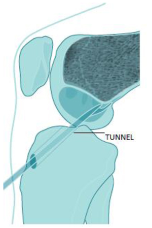
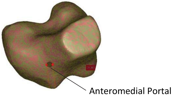
Anteromedial Portal (AMP) techniques are most commonly used for anatomical Anterior Cruciate Ligament Reconstruction along with Traditional Transtibial (TT) technique reconstruction. In Traditional Transtibial technique Anterior Cruciate Ligament femoral tunnel is drilled through tibia tunnel positioned in the posterior half of the native Anterior Cruciate Ligament tibial attachment site. The ability of Transtibial technique to recreate anatomy and function of Anterior Cruciate Ligament was questioned by many researchers which led to the use of Anteromedial Portal Technique. The comparison between Traditional Transtibial and Anteromedial Portal Techniques is shown in Figs. (1a, 1b).
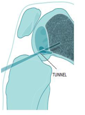
In the Anteromedial Portal technique described by Charles Brown Jr [6], the ACL femoral tunnel is drilled through an accessory anteromedial (AAM) portal with the knee flexed to 120° or higher. The femoral tunnel position is more accurately specified by using any of the following foot print measurement techniques: ACL ruler, Lateral Inter Condylar and Bifurcate Ridges, native Anterior Cruciate Ligament, Intra–operative Fluoroscopy techniques.
Wang et al. [7] have compared AMP & TT techniques based on the clinical outcome of the ACL reconstruction surgery and they have reported the AMP technique to be more effective than TT technique in restoring anterior–posterior translation and internal–external rotation. But, they have not used finite element method for comparing the two techniques. Finite element method for comparing these two techniques of anatomic ACL reconstruction causes least hinderances to daily life of the subjects under study. This study utilizes Magnetic Resonance Imaging (MRI) of patients for analysis. Hence, the subjects need to come in person for the study. This not only reduces study time, but also gives effective results without causing any embarrassment to the patient and does not require disruption of daily activity of the patient during physical examination at the time of the study.
2. MATERIALS AND METHODS
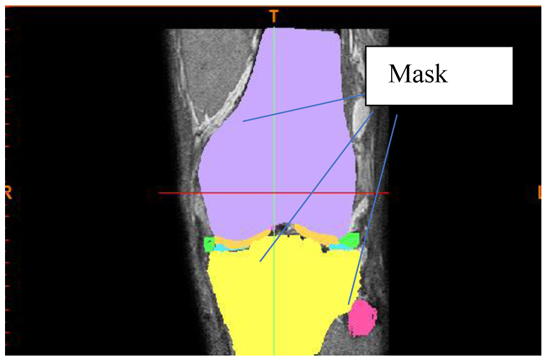
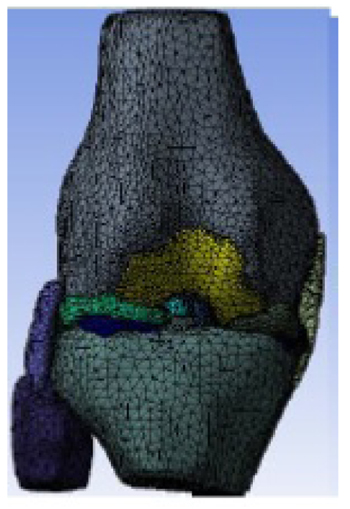
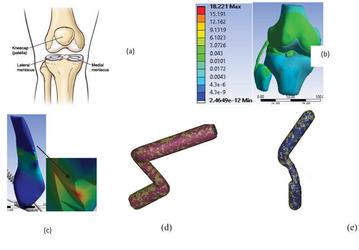
Four healthy persons in the age group of 17 to 35 years were considered for the study. Their MRIs were utilized for this study. MRIs were converted into 3–Dimensional (3D) models using MIMICS (Materialise Inc., Leuven, Belgium) software in Digital Imaging and Communications in Medicine (DICOM) format. The stacked DICOM images were collated so that 3D geometry can be generated. The first step in the process is the generation of a 2 – Dimensional surface called ‘Mask’ on each slice of the MRI (Fig. 1c). From these ‘Masks’ the individual parts of knee joint were generated. Subsequently, these parts were assembled to obtain the geometric model of the joint.
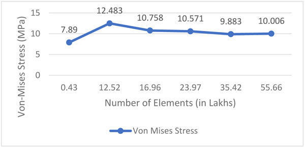
The geometric model of the joint was exported to 3–matic (Materialise Inc., Leuven, Belgium) software where it was converted into a finite element model using 10 – node (second–order) tetrahedral element. Firstly, the surface mesh was carried out followed by volume mesh of the individual parts of knee joint. The finite element model of the human knee joint belonging to one of the five subjects is shown in Fig. (1c). The appropriate number of elements was decided by carrying out the grid independence test. This was done by varying the number of elements from 43,203 to 55,66,069. Altogether six instances of different number of elements with as many sequential instances of different sizes of elements were considered in this range of number as indicated in Fig. (1d). The grid–independence test was carried only on the first subject; the optimum number of elements obtained from this was utilized for subsequent subjects. Then the finite element models were exported to ANSYS (Ansys Inc., USA) workbench for further analysis.
The number of subjects was determined based on statistical significance [8] given by Eqn. (1).
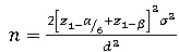 |
(1) |
Where, z1-a/6 = 2.39 at α = 0.05/3 (adjusted for three comparisons)
z1-β = 0.84 at 80% power
σ2 = common assumed variance = 32 [9]
d = clinically important difference = 7 [10]
Therefore, n = 4 per group.
ACL reconstruction was simulated on four human subjects with healthy knee joints as in Table 1.
| Subject | Gender | Age |
|---|---|---|
| 1 | Male | 17 |
| 2 | Male | 31 |
| 3 | Male | 32 |
| 4 | Male | 35 |
Table 1 gives description about the gender and age of the subjects whose MRI is used for analysis and reconstruction. The age and gender were based on the availability of MRI for research at the clinical repository.
2.1. Modeling
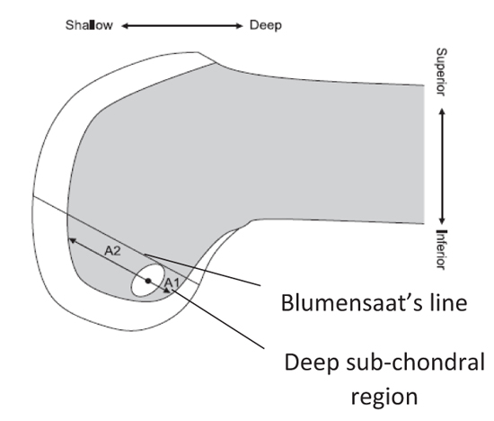
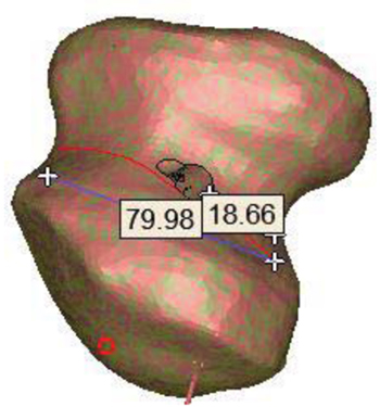
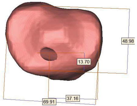
Femoral and Tibial foot prints were marked in 3 – matic (Materialise Inc., Leuven, Belgium) as per the anatomic ACL reconstruction requirements. As seen in Fig. (2a), the central point of the femoral tunnel was calculated as A1/(A1+A2) using Mochizuki’s method [11]. Where, A1 is the distance between the deep subchondral margin and the central point of the tunnel along Blumensaat’s line which is the line drawn along the roof of the intercondylar notch of the femur as seen on lateral radiograph of the knee joint [11]. In this study, the femoral foot print was located based on Mochizuki’s method at 38.7 ± 2.7% from the deep subchondral margin as seen in Fig. (2c).
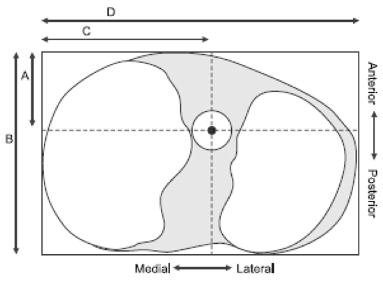
As seen in Fig. (2b), the central point of the tibial tunnel from the anterior and medial edges of the tibial plateau was calculated as A/B and C/D respectively using Tsukada’s method [11]. Where, A: distance between anterior tangential line and central point of tibial tunnel, B: distance between anterior and posterior tangential lines, C: distance between medial tangential line and central point of tibial tunnel, D: distance between medial and lateral tangential lines. The mean tibial tunnel position was located such that A is 44.6 ± 2.5% posterior of B from the anterior margin and C is 48 ± 3% lateral of D from the medial margin. The central point of tibial tunnel was located using Tsukada’s method as shown in Fig. (2d). This process was continued on knee joints of subjects 2, 3 and 4. AMP technique will be represented as Case – A and TT technique will be represented as Case – B in this paper further.
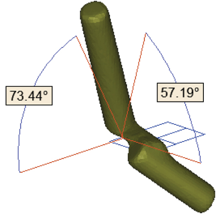
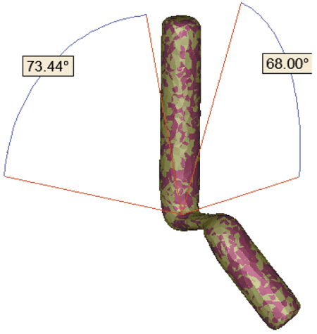
s were drilled in the knee joints of all the subjects at the tibial and femoral foot prints, Fig.(2c) and 8 show the opening of the holes in the femur and tibia respectively for subject–1. The obliquity of femoral holes was in the range of 69 to 76 degrees in the coronal view and in the range of 51 to 58.5 degrees in the sagittal view as per AMP technique [12] (Case–A). Similarly, coronal obliquity of the graft in the femoral tunnel was in the range of 72 to 78 degrees and sagittal obliquity was in the range of 59 to 69.5 degrees as per TT Technique [13] (Case–B). The angles are measured with respect to tibial plateau/axial plane [12].
Figs. (3a, 3b) represent femoral obliquity of Reconstructed – ACL (R – ACL) in sagittal and coronal planes when fixed inside the femoral and tibial holes after reconstruction. The R – ACL with tibia screw is shown in Fig. (3c). Similar process is followed for the other subjects. In the present work, hamstring tendon graft of 9 mm diameter was considered as per standard surgical practice [10].
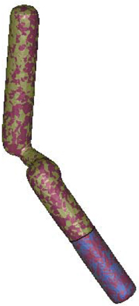
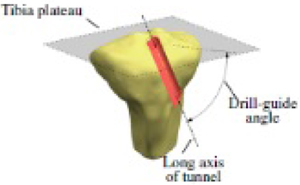
In case – A, an anteromedial portal of 4.5 mm diameter with a depth 4 mm is drilled in the superior side of femur, 10 mm below this hole tip of hamstring tendon graft is placed. Fig. (3d) shows anterior–superior view of the femur from which shallow region of anteromedial portal can be seen. But, this feature is absent in case – B. The tibial drill–guide angle for Cases A & B were chosen to be 45 degrees in the sagittal plane for all the subjects as it is close to the values chosen by surgeons [5]. It is shown in Fig. (3e).
The model is meshed with 10 – node tetrahedron element in 3 – matic (Materialise Inc., Leuven, Belgium). This element has three degrees of freedom in translational mode. The total number of elements in each of the subject is between 23,97,000 to 30,00,000 elements in the finite element model. The number of elements is obtained from grid independence test as in Fig. (1d). A meshed of the healthy and ACL reconstructed knee joint model is shown in Fig. (4a) is exported to ANSYS (Ansys Inc., USA) workbench for further analysis.
2.2. Lachman Test Loading
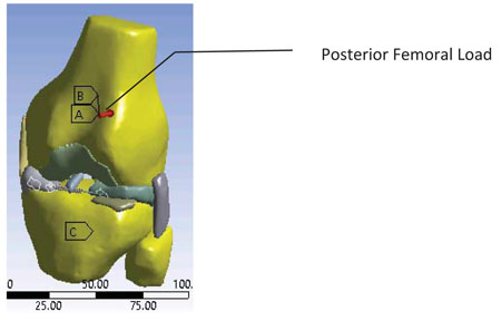
A 134 N [12] load is applied to the joint in the anterior – posterior direction for estimating Posterior Femoral Translation (PFT) or Anterior Tibial Translation (ATT) and the Equivalent (Von – Mises) stress distribution in the model. As per the clinical practice, the intactness of ACL is ensured if the ATT is in the range of 5 – 10 mm, i.e. up to a grade – II injury of ACL. The magnitude and direction of this force is derived from KT – 1000c performed on human knee joint. A 134 N posterior directional load was applied on the centroid of the femur as shown in Fig. (4b) where it is represented by condition – B. In the knee joint as shown in Fig. (4b) boundary condition – A in which femur is free to translate in all degrees of freedom with degrees of rotation being fixed and condition – C in which tibia and fibula are free to rotate in internal – external rotation, valgus – varus rotation. The contacts are of either bonded or no–separation type. The loads and boundary conditions remain same for healthy knee joint and knee joint with simulation of ACL reconstruction.
3. RESULTS
The mean value of stress and standard deviation are 13.934 MPa and 5.1 MPa respectively (Table 2) for healthy human knee joints.
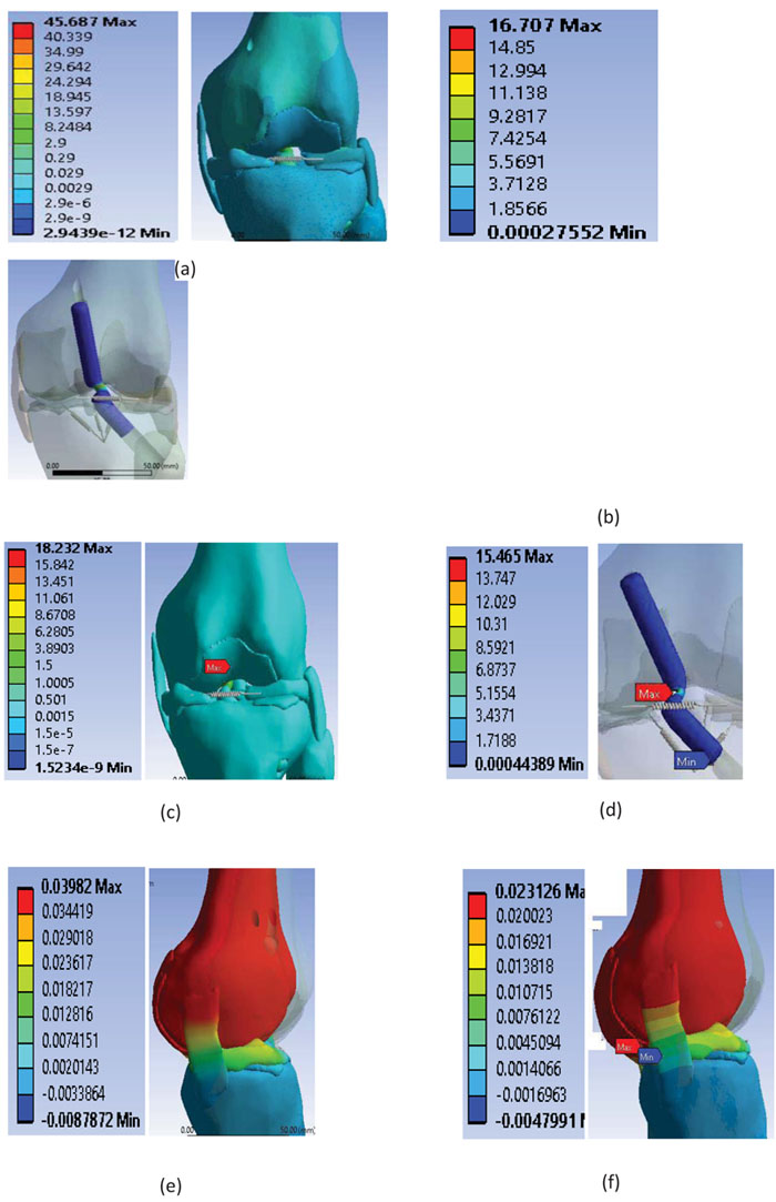
The results of Posterior Femoral Translation (PFT) and the stress distribution in the four knee joints subjected to simulation of ACL reconstruction are shown in Figs. (5 to 9). In subject–1, case–A the stress (maximum Von-Mises stress) induced in the joint is 45.687 MPa and the same in the R – ACL is 16.7 MPa at its femoral insertion as shown in Figs. (5a) and (5b). Stress of 18.23 MPa is observed in the knee joint for Case – B as seen in Fig. (5c) and a stress of 15.47 MPa is observed in the R – ACL as in Fig. (5d). Posterior femoral displacement of 0.039 mm and 0.023 mm are observed in the femur for Cases A and B respectively, as shown in Figs. (5e,f).
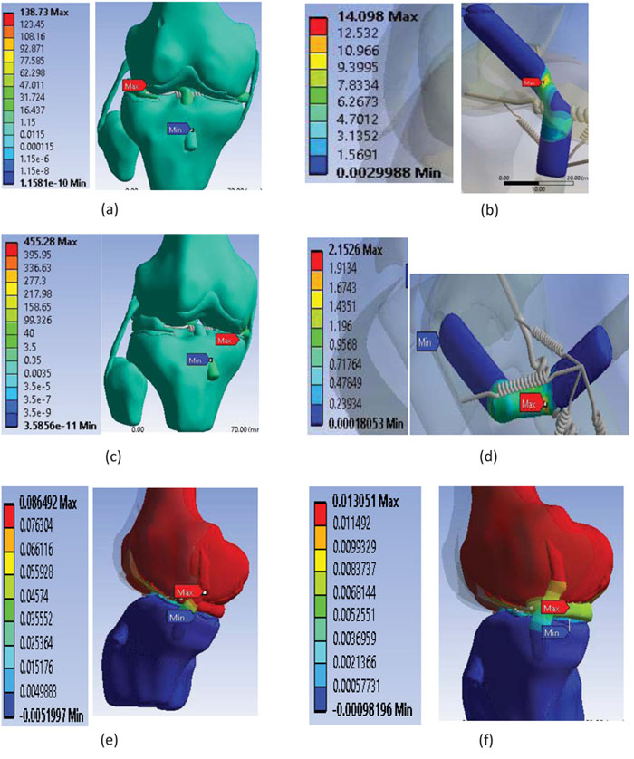
In subject – 2, Case – A showed the stress of 138.73 MPa in the joint as seen in Fig. (6a). The stress of 14.09 MPa occurred in the R – ACL at its femoral insertion as indicated in Fig. (6b). For the same subject, the stress of 455.28 MPa is observed in the knee joint for case – B as seen in Fig. (6c) and a stress of 2.153 MPa is observed in the R – ACL near the articulating region of the knee joint as observed in Fig. (6d). Posterior femoral displacement of 0.087 mm and 0.013 mm are observed in the femur for Cases A and B respectively as seen in Figs. (6e,f).
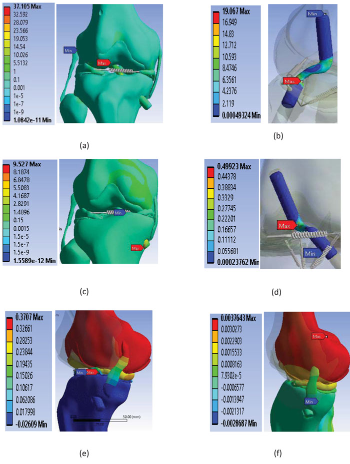
In subject – 3, case – A showed the stress of 37.1 MPa in the joint as depicted in the Fig. (7a) and the stress of 19.07 MPa occurred in the R – ACL at the femoral insertion as seen in Fig. (7b). Whereas the stress of 9.53 MPa is observed in the knee joint for Case – B as seen in Fig. (7c) and a stress of 0.5 MPa is observed in the R – ACL as indicated in Fig. (7d). Posterior femoral displacement of 0.37 mm of 0.037 mm are observed in the femur for Cases A and B respectively as evident in Figs. (7e,f).
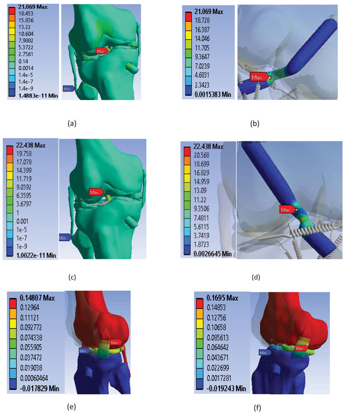
In subject – 4, case – A showed the stress of 21.07 MPa in the joint as seen in Fig. (8a) and the stress of 21.07 MPa occurred in the R – ACL at its femoral insertion as depicted in Fig. (8b). Further, the stress of 22.44 MPa is observed in the knee joint for Case – B as indicated in Fig. (8c) and the stress of 22.44 MPa is observed in the R – ACL as appeared in Fig. (8d). Posterior femoral displacement of 0.149 mm and 0.169 mm are observed in the femur for Cases A and B respectively as observed in Figs. (8e,f).
rom the results of the analysis it can be observed that the stress occurs either at the tibial or at the femoral insertion. The insertions of hamstring tendon graft in the femur and tibia were up to maximum possible length, hence producing maximum possible fixation to the bones [11]. In subjects 2 and 4, Case – B has higher stress in the knee joint when compared to case – A. Whereas, in subjects 1 and 3, case – B has lower stress in the knee joint when compared to case – A.
Table 3 shows stress and displacement in the human knee joint which has undergone ACL reconstruction by AMP and TT techniques. Stress in the Reconstructed – ACL (R – ACL) for all subjects except subject 4 is higher for AMP technique when compared with TT technique. In AMP technique stresses in the R – ACL is comparable with stress in the ACL of healthy knee joint (Table 2). But, this is not true for TT technique.
4. DISCUSSION
It is observed that in Tables 2 and 3 for case-A (AMP technique), stress varies with orientation of ACL for both intact and reconstructed conditions of the same subject during Lachman test. It is also observed that R – ACL shows stress (maximum von – Mises) in the articulating region of the knee joint among all the subjects. In subject – 1, intact ACL has an obliquity of 21.77° and 0° in the sagittal and coronal planes respectively with a stress response of 6.76 MPa whereas, R – ACL has an orientation of 32.28° and 101.86° in the sagittal and coronal planes respectively with a stress of 16.71 MPa. Thus, the stress induced in ACL increases by 147%. The significant difference in stress induced in ACL between intact and reconstructed conditions is mainly due to huge difference in coronal obliquity of ACL. It may also be noted that the obliquities of reconstructed ACL in both sagittal and coronal planes are higher than that of intact ACL. Subject – 2 experienced a stress of 18.22 MPa and 14.1 MPa for intact and reconstructed conditions respectively. In this subject there is a decrease of stress in ACL by 22.5%. In this subject, the obliquities of intact ACL in sagittal and coronal planes are 40.68° and 63.06˚ respectively whereas; the obliquities of R-ACL in sagittal and coronal planes are 16.1˚ and 7.52˚ respectively. Further, it is observed that the obliquities of R – ACL in sagittal and coronal planes are smaller than that of intact ACL. In Subject – 3, magnitude of stress in R – ACL (Table 3) in AMP technique is comparable with that of intact ACL (Table 2). The obliquities of intact ACL in sagittal and coronal planes are 45.02˚ and 18.55˚ respectively whereas; the obliquities of R – ACL in sagittal and coronal planes are 35.64˚ and 55.94˚ respectively. It may be noted that the obliquity of R – ACL in sagittal plane is smaller when compared with intact ACL whereas; the obliquity of the same in coronal plane is higher than that of intact ACL. In subject – 4, the intact ACL has an obliquity of 44.36° in the sagittal plane and 7.78° in the coronal plane exhibiting a stress of 8.84 MPa. Whereas, R – ACL has a stress of 21.07 MPa with an orientation of 74.06° and 21.84° in the sagittal and coronal planes respectively. The stress induced in R – ACL increases by 138% when compared with that of intact ACL. It is also observed that the obliquities of R-ACL are more than that of intact ACL in sagittal and coronal planes. This implies that the stress increases with increase in angle of orientation of ACL. During Lachman test the load is applied on femur in anterior – posterior direction. ACL originates from the anteromedial part of tibia and gets connected at posterolateral part of femur and hence it is generally inclined to both sagittal and coronal planes. Therefore, the load applied during Lachman test causes both bending and axial effects on ACL. It is also true that for a given load the bending stress induced in ACL is more than the axial stress. Further, the bending effect becomes more and more dominating the axial effect with the increase in angle of orientation of ACL.
| Subject | Age |
Stress in ACL (Location) |
Stress in Knee Joint (Location) |
Angle Projected on Plane (measured from XY plane) | |
|---|---|---|---|---|---|
| Sagittal plane | Coronal plane | ||||
| 1 | 17 | 6.76 (F.I) | 8.25 (Fibula-LCL) | 21.77 | 0 |
| 2 | 31 | 18.22 (M.S) | 18.22 | 40.68 | 63.06 |
| 3 | 32 | 19.08 (M.S) | 21.83 (Femur-ACL) | 45.02 | 18.55 |
| 4 | 35 | 16.77 (M.S) | 61.19 (Femur-ACL) | 40.84 | 10.4 |
| 5 | 33 | 8.84 (M.S) | 8.84 | 44.36 | 7.78 |
| S | Stress | Displacement | Articular region angle (degrees) | |||||||
|---|---|---|---|---|---|---|---|---|---|---|
| AMP (Case–A) | TT (Case–B) | AMP (Case–A) | TT (Case–B) | AMP (Case–A) | TT (Case–B) | |||||
| Knee Joint | R – ACL | Knee Joint | R – ACL | Sagittal | Coronal | Sagittal | Coronal | |||
| 1 | 45.69 | 16.71 | 18.23 | 15.47 | 0.04 | 0.023 | 32.28 | 101.86 | 76.2 | 15.79 |
| 2 | 138.73 | 14.1 | 455.28 | 2.15 | 0.08 | 0.013 | 16.1 | 7.52 | 43.57 | 43.49 |
| 3 | 37.1 | 19.07 | 9.53 | 0.5 | 0.37 | 0.0037 | 35.64 | 55.94 | 115.7 | 10.86 |
| 4 | 21.07 | 21.07 | 22.44 | 22.44 | 0.15 | 0.17 | 74.06 | 21.84 | 57.75 | 31.73 |
From the results presented in Table 3, it is found that the mean value of maximum Von–Mises stress in the R – ACL for AMP technique was 17.74 ± 3.01 MPa. In subjects 1 and 4, mean stress in the intact ACL and stress in the R – ACL (cases A and B) are comparable (Tables 2 and 3). In subjects 2 and 3, stress in the R – ACL is comparable to stress in the intact ACL (Table 2) for only case – A whereas, stress in the R – ACL for Case – B is much lower than means stress of the intact ACL. This implies that despite ACL foot prints and orientations conforming with the recommended ranges, in subjects 2 and 3 the R – ACLs in case – B are not able to replicate the anatomic position and orientation of intact ACL. Therefore, patient specific ACL reconstruction procedure must be undertaken for these subjects as per the principles of anatomic ACL reconstruction [12]. Considering case – A, all the subjects show stress in the R – ACL (Table 3) to be comparable with the mean stress of the intact ACL in the healthy human knee joint (Table 2). Whereas, in case – B not all subjects show stress in the R – ACL (Table 3) to be comparable with the mean stress of the intact ACL in the healthy human knee joint (Table 2). This shows that it is not consistently possible to place the reconstructed ACL to its anatomical position and orientation by TT technique. Hence, AMP technique with which it is consistently possible to place the R – ACL to its anatomic position and orientation is better than TT technique in fulfilling principles of anatomic method of ACL reconstruction.
It is observed that the knee joint of subject – 2 has highest stress (Table 2) among all the subjects. The maximum stress in subject – 2 is at the cartilage – menisci interface. It is to be noted that the medial meniscus of subject – 2 is shorter than that of the same in an ideal knee joint in the anterior region (Figs. 9a, b). In addition to this, ACL of subject – 2 has the highest angle of orientation with tibial plateau in the articular region of the knee joint among all subjects (Table 2). It can also be seen that in subject – 2, the highest stress (Table 2) in the healthy knee joint (Fig. 7c) occurs at its ACL unlike other subjects considered in this study, implying that it is the most important resisting member of this knee joint. After ACL reconstruction using AMP technique this feature of subject – 2 appears to be altered due to significant decrease in its orientation in sagittal plane (Figs. 9c,d,e) when compared with the orientation of ACL in healthy joint (Table 2). This could make the reconstructed ACL more of axially loaded member than before and thereby causing bulk of the load to be taken up by the joint. Due to this reason, after reconstruction using AMP technique the stress in knee joint of subject – 2 is far more than all other subjects. Whereas, in case – B (TT technique) the stresses induced in ACL and the joint are highly inconsistent (Table 2). In addition to this, there appears to be no correlation between the orientation of reconstructed ACL and the stress induced. Hence, it could be one of the reasons for considering TT technique inferior to AMP technique [6].
In the present study, MRIs of healthy knee joints were utilized to simulate the anatomic ACL reconstruction in the knee joint. Very few researchers have quantitatively compared AMP and TT techniques of single bundle ACL reconstruction. Among them, Wang et al. [6] have quantitatively compared the two techniques by post–operative examination of patients. In their study, they have found that AMP technique is better than TT technique during single bundle ACL reconstruction. But, these researchers had come to this conclusion after physically examining the patients during follow up after reconstruction. Therefore, it was mainly on the basis of clinical assessment without taking much of the assistance from quantitative tools. This process of comparing AMP and TT techniques demands a lot of time and effort from the patient, orthopaedician and the researcher for the study. Apart from this, it may also cause inconvenience to the patients during the study. But, the process followed in the present study not only avoids the clinical examination of the patients after reconstruction for the purpose but also generates a lot of quantitative results which come in handy for the drawing conclusions. It does not cause any inconvenience to the patients as the study is offline which uses the readily available MRIs from the hospital repository.
However, this study is limited to Indian male subjects. The future scope lies in utilizing subjects from different ethnic backgrounds. Also, both male and female subjects may be considered in future for the study to understand the influence of gender if any, on the outcome. In the present study, only Lachman test loading is considered. In future, different human activities and knee joint flexion positions along with corresponding loading conditions may be considered for the study.
CONCLUSION
Based on the result of the analysis following conclusions were made:
- Despite using anatomic method of ACL reconstruction for the simulation; Traditional Transtibial (TT) technique when compared with Anteromedial Portal (AMP) technique either produces severe stress (subjects 2 and 4) or comparable stress in the knee joint.
- Knee joint reconstructed by AMP technique produces stress and displacement which is comparable to that of healthy knee joint. Whereas, the knee joint which has undergone ACL reconstruction by TT technique produces very high stress in the knee joint and very low stress in the R – ACL.
- There are some instances (subjects 1 and 4) in which stress in the R – ACL is comparable for both AMP and TT techniques. This may be due to the specific combination of anatomic positioning of femoral foot – print and femoral and tibial obliquities in these joints.
- The Posterior femoral displacement of the knee joint which have undergone TT technique are lesser than AMP technique in subjects 1,2 and 3. From this it can be observed that ACL reconstruction by TT technique makes the joint more rigid when compared to AMP technique.
ETHICS APPROVAL AND CONSENT TO PARTICIPATE
The study was approved by the Communication of the Decision of the Institutional Ethics Committee (Registration No. ECR/146/Inst/KA/2013).
HUMAN AND ANIMAL RIGHTS
No Animals were used in this research. All human research procedures followed were in accordance with the ethical standards of the committee responsible for human experimentation (institutional and national), and with the Helsinki Declaration of 1975, as revised in 2008.
CONSENT FOR PUBLICATION
Not applicable.
CONFLICTS OF INTEREST
The authors declare no conflict of interest, financial or otherwise.
ACKNOWLEDGEMENTS
The authors thank Dr. Issay Narumi for valuable comments.