Characterizing and Evaluating Cell Specialization Through the Gini Index of Gene Expression: A TCGA Normal vs. Tumor Case Study
Abstract
Introduction
The Gini index, introduced by the Italian statistician and demographer Corrado Gini in the first decades of the 1900s, is commonly used as a measure of statistical dispersion to evaluate income inequality within a nation. However, it is a powerful and effective measure to characterize any sample distribution and evaluate how far it is from a uniform one.
Methods
In this work we used the Gini Index as an effective and reliable measurement of the specialization of cells, using it to evaluate and compare the specialization level of normal and tumor cells according to their gene expressions.
Results
It turned out that, on average, tumor cells tend to lose their specialization or, in other words, their capacity to be the cells they were intended to be due to cancer effects. This loss of specialization in tumor cells corresponds, in our analysis, to a lower Gini Index with respect to normal cells. This behavior was observed both at a single patient level comparing Gini Indexes of coupled samples (from the same patient) and at a global level comparing distributions of Gini Indexes in normal and tumor datasets.
Discussion
This work demonstrates that the Gini Index (GI) effectively captures the loss of transcriptional specialization in tumor cells compared to normal tissues, with statistically significant differences observed both within patients and across cancer types, despite some exceptions, such as KICH and THCA.
Conclusion
In conclusion we are confident that GI could be a valuable and effective parameter to evaluate cell specialization and could provide significant insights in the context of cancer studies.
1. INTRODUCTION
The Gini index (GI) was introduced by the Italian statistician and demographer Corrado Gini in the first decades of the 1900s [1-3]. It is commonly used as a measure of statistical dispersion to evaluate income inequality within a nation. The general principle is based on the comparison between the portion of economic resources and the portion of the population that possesses those resources. In other words, the GI measures how the distribution of any source of data deviates from being uniform, collapsing this information into a number ranging from 0 to 1. In a country where a small number of individuals are extremely wealthy while the vast majority are extremely poor, the Gini Index (GI) is very high and approaches 1. Conversely, the Gini Index (GI) is very low—approaching 0—in a country where the majority of people have similar or comparable incomes. Although the GI was introduced and commonly used in this context, it can be applied to any distribution to investigate how far it is from being a uniform distribution. The GI provides information that is associated with but also complementary to other measures, such as the standard deviation or entropy, but it has several advantages, such as the direct comparability of any set of data since it is a number in the range [0,1]. Moreover, it does not need any kind of assumption as in the case of entropy, where, in most cases, a binning supervised pre-process is necessary. Jiang and colleagues in 2016 developed GiniClust, a tool that uses the GI in a biological context to characterize rare cell types in single-cell experiments [4]. In 2018, Tsoucas and Yuan developed a new tool, GiniClust2, that improved the ability to detect and cluster different cell types in single-cell experiments [5]. In 2021, Nguyen and colleagues developed the Polar Gini Curve method to characterize cluster markers by analyzing single-cell RNA sequencing data [6]. The GI was also used to characterize and identify gene classes, for example, housekeeping as well as Transporter genes according to their expression variability across different cells [7, 8], to select genes for normalizing expression profiling data or in combination with Support Vector Machines to select informative genes that improve the effectiveness of classification [9, 10].
In 2024, Furth and colleagues evaluated epigenetic heterogeneity using GI to demonstrate how oncogenic IDH1mut drives the loss of histone acetylation and increases chromatin heterogeneity [11]. In immunoinformatics, GI has been shown to be an effective measure for evaluating diversity in single-cell T-cell and B-cell receptor sequencing experiments [12-14]. Additionally, GI has been applied in various biological contexts as an attribute selection metric in decision trees and random forest algorithms [15-17].
To the best of our knowledge, this work is the first attempt to apply the GI to gene expression in the context of tumors, comparing the GI of normal and tumor cells and evaluating their cell specialization.
In this work, we introduce the GI as an effective and reliable measurement of the specialization of cells, using it to evaluate and compare the specialization level of normal and tumor cells according to their gene expressions. The statistical significance of the differences between tumor and normal GI values was evaluated through hypothesis tests both at a single-patient level comparing GIs of coupled samples (from the same patient) and at a global level comparing distributions of GIs in normal and tumor datasets.
2. METHOD
We focus on the public gene expression (FPKM - Fragments Per Kilobase of transcript per Million mapped reads) quantification experiments of the TCGA program available on the open-access OpenGDC repository [18, 19] for running our analyses. Here, every kind of experimental data and metadata is first extracted from the Genomic Data Commons portal [20, 21], and then standardized into the free-BED format whose structure is described in the OpenGDC Format Definition documentation available at http://geco.deib.polimi.it/opengdc/.
The gene expression quantification data contain the list of genes involved in the experiments with their genomic coordinates (defined as chromosome, start position, end position, and strand) and their quantitative information like the htseq-count (number of reads mapping to a specific gene), FPKM (Fragments Per Kilobase of transcript per Million mapped reads – it normalizes the read count based on gene length and the total number of mapped reads), and FPKM-UQ (same as FPKM but considering the upper quartile only).
In this study, we focus on 17 out of 33 different tumor types (see Abbreviations section for the complete list of considered tumor types) available in the OpenGDC database, considering a number of paired normal-tumor samples ranging from a minimum of 9 (ESCA) to a maximum of 112 (BRCA). The number of samples for each tumor type is reported in Tables 1 and 2.
For each cancer type and each patient, we compare paired normal and tumor gene expression GIs to assess whether they differ significantly. To this end, the actual observed difference between normal and tumor GIs is compared with a distribution of 1,000 artificial GI differences generated by randomizing gene expressions of the two samples. Specifically, for a given cancer type, we build the set of samples P={p1, p2,.. pn} for which both normal and tumor gene expressions are available. The GIs of gene expression associated with each pi are indicated with GIiT and GIiH for normal and tumor samples, respectively. We define it as GID(pi) = GIiH-GIiT : the difference between normal and tumor GIs. We then determine whether GID (pi) value is statistically significant or, in other words, whether the observed value can attest that the two conditions show significantly different gene expression distributions when evaluated through the GI. The GID(pi) is a pure number that, in general, depends on the two distributions, so we have to compare it with an expected value obtained by taking the two distributions into consideration. We generate artificial pairs of random gene expression vectors by shuffling the two gene expression vectors. For each gene, we randomly associate to the first vector one out of the two gene expression values and we assign the other value to the other vector. Once the two randomized vectors are obtained, we compute the correspondent GIs, namely GIiHR and = GIiTR and finally GIDR(pi) = GIiHR-GIiHT We iterate this procedure 1,000 times, obtaining a collection of 1,000 GIDR(pi) and we then compute the z-score as:
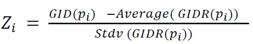
|
where Average (GIDR(pi)) and Stdv (GIDR(pi)) are the average and the standard deviation of the 1,000 obtained GIDR(pi). According to the Shapiro-Wilk normality test, performed on sample cases (data not shown), the distribution of GIDR(pi) can be considered to be extracted from a normal distribution, allowing us to compute the P-value from a given z-score. We compute P-values considering separately the two tails of the normal distribution, evaluating the p-value for both tails when the normal GI is greater than the tumor one and vice versa when the normal GI is smaller than the tumor one. We set a P-value threshold of 0.01, applying the Bonferroni correction with respect to the number of samples of the considered tumor type.
At the end of this procedure we obtain for each tumor type and each patient a P-value indicating whether the normal and tumor expression values are significantly different from a statistical point of view when evaluated through the Gini indexes. A significant P-value derived from a positive z-score is associated with a positive difference, indicating that normal GI is significantly greater than tumor GI. In this case, normal cells are more specialized than tumor cells. On the other hand, a significant P-value derived from a negative z-score is associated with a negative difference, indicating that normal GI is significantly smaller than tumor GI.
For each cancer type we also compare paired normal and tumor gene expression GI distributions. To establish whether they come from the same hypothetical distribution, we perform paired Wilcoxon tests. The Bonferroni adjustment is applied for multiple test corrections. Finally, we compare normal and tumor GI distributions for all available samples, including unpaired ones (samples for which only one condition is available). Unpaired Wilcoxon tests and the Bonferroni adjustment are applied in the same way.
The entire procedure is repeated using the standard deviation (STDEV) of gene expression values, instead of the Gini Index (GI), to enable comparison at both the individual patient level and the global level.
3. RESULTS
The main goal of this paper is to study cell specialization through the GI index of gene expression comparing cancer and normal cells. First, we present a global view of GI values associated with samples coming from patients with different cancer types (see Abbreviations section) for both normal and tumor cells. We then analyze and compare for each single patient, normal and tumor GIs, showing through z-score values that they are mostly significantly different. Then, we study and evaluate for each tumor type the statistical differences between normal and tumor GI distributions through Wilcoxon tests. We apply paired statistical tests to compare GI distributions of normal and tumor-coupled samples. Finally, we consider a broader dataset including all available samples, even if not coupled, by applying non-paired statistical tests.
Table 1 reports a global view of GI values for each tumor type. The first column indicates the tumor type, the second column indicates the number of subjects for which both normal and tumor samples are available. The other columns show other statistical parameters related to GI distributions. GI values are typically distributed around 0.9, with the average in normal samples ranging from 0.907 in BRCA to 0.969 in LICH, while in tumor samples, from 0.906 in LUSC to 0.951 in LICH.
Fig. (1) shows the comparison between GI distributions of tumor (orange) and normal (blue) cells for four different cancer types. Panel A – on the left side of the figure – (HNSC and LIHC) clearly shows higher GI values for normal samples compared to tumor samples. On the other hand, panel C – right side of the figure – (THCA) shows an opposite behavior with higher values for tumor samples. Panel B (PRAD) shows an intermediate case where there is no clear prevalence between tumor and normal samples. Most of the tumor types typically show GI values that are lower in cancer than in normal samples (see Supplementary Material S1 – Supplementary Tables S1.1-17 – for a complete view of GI distributions of all the cancer types).
In order to statistically evaluate the significance of this observed difference at a patient level, we compare the difference between tumor and normal GIs with the difference distribution between artificial gene expression arrays randomly generated from the actual ones obtaining a z-score value and the corresponding P-value (see Materials and Methods).
In Table 2, the number and percentage of patients showing a significant positive difference between normal and cancer cells are reported in column 3 for each tumor type. In the same way, columns 4 and 5 report the numbers and percentages of non-significant and significant negative GI differences, respectively. The rows corresponding to a given tumor type are highlighted in green (red) when the majority of patients show a significant positive (negative) difference (P-value < 0.01). In the same Table 2, + and - symbols indicate the statistical significance of the Wilcoxon rank-sum test performed on all the normal and tumor samples regardless of their pairing (see Method Section). A + symbol denotes that normal GI values are significantly higher than tumor GI values considering a Bonferroni adjusted p-value<0.01, while a - symbol denotes that normal GI values are significantly smaller than tumor GI values. The two analyses lead to, as expected, similar and consistent results, even if they provide a different view at a patient level and a global level.
Wilcoxon tests are also performed on the GIs distributions of paired samples for each tumor, obtaining the same results except for LUSC and ESCA, which are found not significant.
We always refer to the different tumor types with their abbreviations as reported on the Genomics Data Commons website (see Abbreviations section for the complete list of tumor types alongside their extended description).
| Tumor Type | Subjects | Summary of Gini Indices | |||
|---|---|---|---|---|---|
| Normal (Average ± Stdev) |
Tumor (Average ± Stdev) |
Normal (Min – Max) |
Tumor (Min – Max) |
||
| BLCA | 19 | 0.926 ± 0.010 | 0.916 ± 0.014 | 0.905 – 0.945 | 0.889 – 0.934 |
| BRCA | 112 | 0.906 ± 0.019 | 0.907 ± 0.016 | 0.873 – 0.966 | 0.878 – 0.971 |
| CHOL | 9 | 0.953 ± 0.003 | 0.917 ± 0.015 | 0.964 – 0.964 | 0.902 – 0.953 |
| COAD | 41 | 0.926 ± 0.008 | 0.917 ± 0.013 | 0.910 – 0.944 | 0.892 – 0.962 |
| ESCA | 8 | 0.937 ± 0.016 | 0.912 ± 0.004 | 0.911 – 0.965 | 0.901 – 0.920 |
| HNSC | 43 | 0.943 ± 0.042 | 0.922 ± 0.014 | 0.907 – 0.972 | 0.887 – 0.960 |
| KICH | 23 | 0.908 ± 0.019 | 0.948 ± 0.015 | 0.880 – 0.932 | 0.909 – 0.974 |
| KIRC | 72 | 0.926 ± 0.027 | 0.916 ± 0.015 | 0.891 – 0.955 | 0.878 – 0.949 |
| KIRP | 31 | 0.924 ± 0.026 | 0.925 ± 0.020 | 0.890 – 0.946 | 0.888 – 0.958 |
| LIHC | 50 | 0.968 ± 0.065 | 0.951 ± 0.012 | 0.953 – 0.983 | 0.914 – 0.975 |
| LUAD | 57 | 0.914 ± 0.021 | 0.909 ± 0.013 | 0.893 – 0.939 | 0.870 – 0.939 |
| LUSC | 49 | 0.913 ± 0.021 | 0.905 ± 0.016 | 0.892 – 0.935 | 0.854 – 0.938 |
| PRAD | 52 | 0.913 ± 0.020 | 0.913 ± 0.016 | 0.871 – 0.956 | 0.879 – 0.978 |
| READ | 9 | 0.919 ± 0.024 | 0.918 ± 0.008 | 0.906 – 0.933 | 0.895 – 0.933 |
| STAD | 27 | 0.945 ± 0.043 | 0.924 ± 0.016 | 0.915 – 0.969 | 0.894 – 0.957 |
| THCA | 58 | 0.908 ± 0.019 | 0.918 ± 0.017 | 0.891 – 0.950 | 0.887 – 0.974 |
| UCEC | 23 | 0.911 ± 0.020 | 0.919 ± 0.02 | 0.893 – 0.924 | 0.881 – 0.965 |
| Tumor Type |
Samples Normal – Tumor (Paired) |
Comparison of Gini Indices for each Patient Through z-score | ||
|---|---|---|---|---|
| Positive (p<0.01) |
Not Significant | Negative (p<0.01) |
||
| BLCA | 19 – 408 (19) | 11 (57.9%) | 6 (31.6%) | 2 (10.5%) |
| BRCA | 113 – 1090 (112) | 34 (30.4%) | 34 (30.4%) | 44 (39.3%) |
| CHOL + | 9 – 36 (9) | 9 (100%) | 0 (0%) | 0 (0%) |
| COAD + | 41 – 456 (41) | 22 (53.7%) | 15 (36.6%) | 4 (9.8%) |
| ESCA + | 11 – 161 (8) | 6 (75.0%) | 2 (25.0%) | 0 (0%) |
| HNSC + | 44 – 500 (43) | 32 (74.4%) | 8 (18.6%) | 3 (7.0%) |
| KICH - | 24 – 65 (23) | 0 (0%) | 1 (4.3%) | 22 (95.7%) |
| KIRC + | 72 – 530 (72) | 35 (48.6%) | 20 (27.8%) | 17 (23.6%) |
| KIRP | 32 – 288 (31) | 9 (29.0%) | 9 (29.0%) | 13 (41.9%) |
| LIHC + | 50 – 371 (50) | 43 (86.0%) | 5 (10.0%) | 2 (4.0%) |
| LUAD | 59 – 513 (57) | 19 (33.3%) | 30 (52.6%) | 8 (14.1%) |
| LUSC + | 49 – 501 (49) | 19 (38.8%) | 23 (46.9%) | 7 (14.3%) |
| PRAD | 52 – 495 (52) | 9 (17.3%) | 27 (51.9%) | 16 (30.8%) |
| READ | 10 – 166 (9) | 1 (11.1%) | 8 (88.9%) | 0 (0%) |
| STAD + | 32 – 375 (27) | 18 (66.7%) | 9 (33.3%) | 0 (0%) |
| THCA - | 58 – 502 (58) | 6 (10.3%) | 20 (34.5%) | 32 (55.2%) |
| UCEC | 35 – 543 (23) | 7 (30.4%) | 5 (21.7%) | 11 (47.8%) |
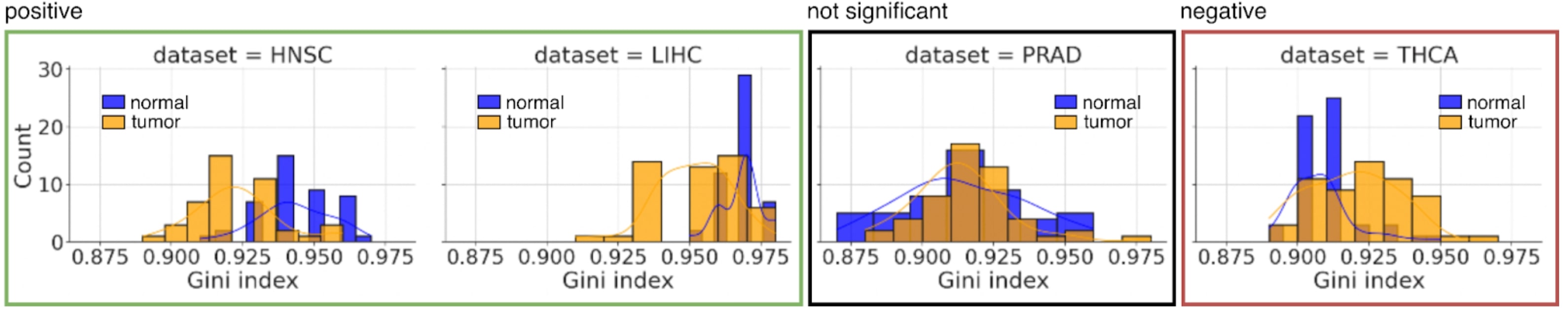
Tumor and normal GI distributions for 4 different tumor types: HNSC and LIHC (panel A, green box), PRAD (panel B, black box), and THCA (panel C, red box). The plots show for each of the 4 considered tumor types how many samples (y-axis), tumors in pink and normal in cyan, have a GI falling in the corresponding bin (x-axis).
Note that we also performed the same statistical analysis of z-scores and Wilcoxon rank-sum test based on the STDEVs instead of GIs, with the aim of proving the effectiveness of GIs over a more classical statistical approach. A summary table of the statistical analysis based on the STDEVs is reported in Supplementary Table S2.1. Also, note that we reported the distribution of the STDEVs alongside the GIs in Supplementary Material S1 – Supplementary Tables S1.1-17. As can be observed by the comparison of Table 2 (GI) and Supplementary Table S1.1-17 (STDEV), similar results are obtained at a global level through Wilcoxon tests (the only differences regard BRCA that is positive and THCA that is not negative for Stdev). On the contrary, the scenario is very different at a patient level; while 7 positives and 2 negatives are found by GI, only 1 positive and 1 negative are found by Stdev. Those results suggest that GI is able to capture the differences in specialization between normal and tumor cells in particular at a single patient level, where Stdev mostly fails.
4. DISCUSSION
As reported in the literature the transcriptional specialization of a tumor is significantly less than the corresponding normal tissue [22]. Consistently, the observed loss of specialization in tumor cells corresponds in our analysis to a lower GI with respect to normal cells. This behavior was observed both at a single patient level comparing GIs of coupled samples (from the same patient) through z-score analysis and at a global level comparing distributions of GIs in normal and tumor datasets.
Interestingly, despite this being the overall typical behavior, few patients show an unexpected increase in their GIs. Similarly, not all cancer types display the same behavior. Some of them, in particular KICH and THCA, show an unexpected increase of specialization in tumor cells (in 95% and 55% of samples, respectively). This astonishing result could suggest that there are peculiar shared patterns between these two tumor types, as reported in a study [23]. One possible reason to investigate further could be a lower tumor mutational burden in THCA and KICH compared to other cancer types, which may affect GI.
It is worth noting that the differences in GI values between normal and cancer cells are comparable to or smaller than the differences among different tissues. Thus, we conclude that the tissue of origin remains more relevant than the tumor or normal condition in determining GI. While one might expect much smaller GI values in tumor samples compared with normal ones, the observed results and statistical analyses (with a significance threshold of P<0.01 and often much smaller P-values) demonstrate that the differences between normal and tumor GIs are highly significant in most cancer types and patients.
The impact and significance of this work may further increase as more data becomes available in TCGA, providing greater statistical robustness and allowing for deeper insights.
CONCLUSION
The GI characterizes a distribution by assessing its deviation from a uniform distribution. It provides information related to, but also complementary to, other statistical measures such as STDEV. In this view it seems particularly suitable to be applied in the context of computational biology. To the best of our knowledge, this work is the first attempt to apply GI to gene expression in the context of tumors, comparing the GI of normal and tumor cells.
We are confident that GI could be a valuable and effective parameter to evaluate cell specialization and could provide significant insights in the context of cancer studies.
AUTHORS’ CONTRIBUTIONS
The authors confirm contribution to the paper as follows: F.C., D.C: Data analysis or interpretaion; All authors reviewed the results and approved the final version of the manuscript.
LIST OF ABBREVIATIONS
The 17 different tumor types considered in this study in the form of study abbreviations are all reported below with their extended name as reported on the official Genomics Data Commons portal at https://gdc.cancer.gov/ resources-tcga-users/tcga-code-tables/tcga-study-abbreviations.
| BLCA | = Bladder Urothelial Carcinoma |
| BRCA | = Breast Invasive Carcinoma |
| CHOL | = Cholangiocarcinoma |
| COAD | = Colon Adenocarcinoma |
| ESCA | = Esophageal Carcinoma |
| HNSC | = Head and Neck Squamous Cell Carcinoma |
| KICH | = Kidney Chromophobe |
| KIRC | = Kidney Renal Clear Cell Carcinoma |
| KIRP | = Kidney Renal Papillary Cell Carcinoma |
| LIHC | = Liver Hepatocellular Carcinoma |
| LUAD | = Lung Adenocarcinoma |
| LUSC | = Lung Squamous Cell Carcinoma |
| PRAD | = Prostate Adenocarcinoma |
| READ | = Rectum Adenocarcinoma |
| STAD | = Stomach Adenocarcinoma |
| THCA | = Thyroid Carcinoma |
| UCEC | = Uterine Corpus Endometrial Carcinoma |
AVAILABILITY OF DATA AND MATERIALS
The results shown here are in whole or part based upon data generated by the TCGA Research Network: https://www.cancer.gov/tcga.
FUNDING
This work has been partially supported by CNR-IASI Project BIOSYS3 – Optimization, models and Algorithms for Bioinformatics and System Science – DIT.AD021.128.
ACKNOWLEDGEMENTS
Declared none.