Early Detection of Neonatal Infection in NICU Using Machine Learning Models: A Retrospective Observational Cohort Study
Abstract
Introduction
Neonatal infections remain a major threat in intensive care units (ICUs), often progressing rapidly and asymptomatically within the first hours of admission. Early detection is critical to improve outcomes, yet timely and reliable risk prediction remains a challenge.
Method
We developed an explainable machine learning retrospective observational cohort study for early prediction of neonatal infection using high-resolution data from the MIMIC-III database. Two-time windows, 30 and 120 minutes post-ICU admission, were analyzed. Physiological and hematological variables were aggregated, and missing data were imputed using Iterative Imputation. We used stratified five-fold cross-validation to test several classification models and feature importance and SHAP analysis to examine model interpretability.
Result
CatBoost demonstrated the best performance in the 30-minute window (F1-score = 0.76), and Gradient Boosting had the best performance in the 120-minute window (F1-score ≈ 0.80). Heart rate, white blood cell count, and temperature were important predictors because they showed both physiological stability and immune response. The 120-minute window made the model work better, indicating the importance of data availability for making accurate predictions.
Discussion
CatBoost at the 30-minute window and Gradient Boosting at the 120-minute window could find a balance between speed and accuracy. Model-based imputation could handle high missing-value rates, but external validation is needed because the data came from only one center and the devices were different.
Conclusion
This study proposes a two-stage decision-support system that adapts to data collected during early and later ICU admission periods. By combining accurate prediction with model interpretability, the framework may enable timely diagnosis and targeted interventions, ultimately reducing neonatal morbidity and mortality.
1. INTRODUCTION
Neonatal infections, including sepsis, remain a leading cause of morbidity and mortality in newborns, particularly in critical care settings, such as neonatal intensive care units (NICUs) [1, 2]. These infections are often difficult to diagnose in their early stages, which requires timely identification to enable effective interventions. Delayed or inaccurate diagnosis can result in rapid disease progression, which increases mortality and long-term complications [3]. Antimicrobial resistance (AMR) has made it even more challenging to treat infections in newborns, making it necessary to use data-driven methods to improve diagnosis and treatment plans [4].
SNAP-II and CRIB are widely used to evaluate neonatal illness severity and predict outcomes as traditional methods [5, 6]. However, these tools are limited by their reliance on fixed variables and retrospective observations, often spanning 12 to 24 hours. They may delay critical decision-making [6] and cannot handle complicated, multidimensional datasets or keep up with changes in patients' conditions [7]. These limitations highlight the need for advanced, real-time predictive tools.
Machine learning (ML) has become a revolutionary method in healthcare because it can combine and analyze complicated data from many different sources [8]. Using machine learning (ML) and deep learning (DL) models like Random Forests, support vector machines, and recurrent neural networks can help make accurate predictions about when a newborn will get an infection and the risks of death that come with it [9, 10]. These models have demonstrated superior performance compared to traditional methods, particularly when applied to large datasets such as MIMIC-III, a publicly available database of critical care patient records [11]. MIMIC-III provides a rich repository of neonatal data, including physiological measurements, laboratory results, and clinical interventions, making it an ideal resource for developing robust predictive models [12].
The goal of this study is to create a machine learning framework that uses data from MIMIC-III to predict neonatal infections and the risks of death that come with them. The proposed method aims to make early, useful predictions by focusing on real-time measurement data gathered during the first few hours of care. This framework will use explainable AI methods to make sure that the predictive models are clear and trustworthy, which will make it easier to use them in clinical workflows. [13]. The outcomes of this research have the potential to enhance early diagnosis, improve resource allocation, and ultimately reduce neonatal mortality in NICUs.
2. METHOD
2.1. Study Design
This research was conducted as a retrospective observational cohort study using the publicly available MIMIC-III Clinical Database (v1.4). The study aimed to address the research question: Can machine learning models applied within the first 30 and 120 minutes of ICU admission accurately predict neonatal infection?
Figure 1 illustrates the overall workflow of the study. A quantitative analytical approach was used. The study population included 6,539 neonates admitted to the NICU, of whom 4,013 were diagnosed with infection. Patients with multiple ICU admissions or those who died within two hours of admission were excluded.
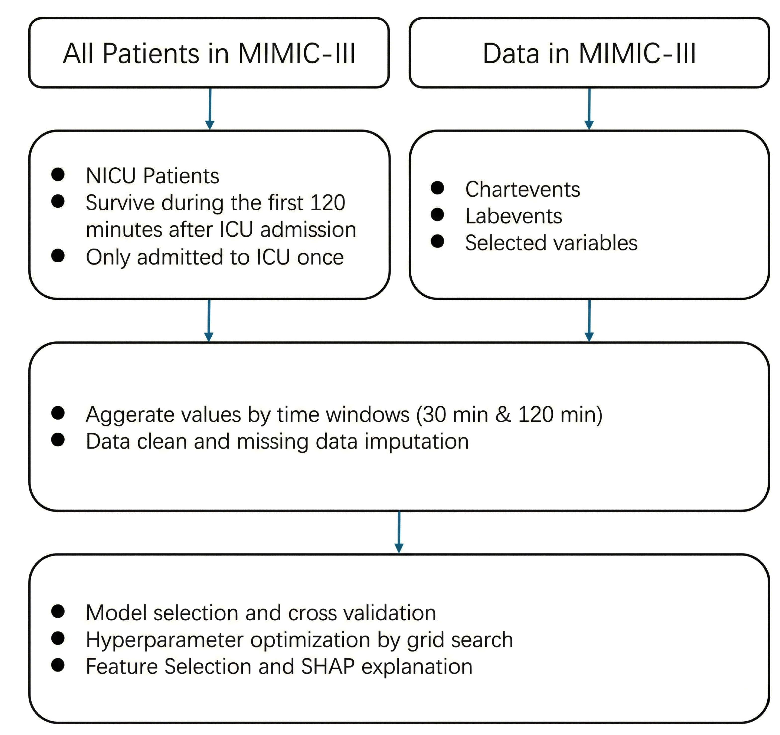
Proposed approach for infection prediction in NICU.
Physiological and hematological variables (e.g., heart rate, respiratory rate, oxygen saturation, temperature, blood pressure, white blood cell counts) were extracted and aggregated into two time windows (30 and 120 minutes post-admission). Data preprocessing included exclusion criteria, variable aggregation, and imputation of missing values.
The study was observational and non-experimental, based on secondary analysis of de-identified clinical data. Multiple supervised machine learning algorithms were evaluated, and performance was assessed using stratified five-fold cross-validation, with F1-score as the primary metric.
2.2. Data Resource
The data source of this retrospective observational study is Medical Information Mart for Intensive Care III (MIMIC-III), a relational critical care database developed by the MIT Lab for Computational Physiology. MIMIC-III is a publicly available dataset containing de-identified health data from patients admitted to critical care units at Beth Israel Deaconess Medical Center. It has detailed health information for 46,520 unique critical care patients who were admitted to the hospital between 2001 and 2013. This includes 58,976 hospital admissions and 38,597 ICU stays. The dataset includes demographics, clinical diagnoses, procedures, medications, lab results, etc. MIMIC-III contains over 2 million chart events, 380,000 laboratory measurements, and over 10,000 procedures, making it a comprehensive dataset for critical care research.
2.3. Data Preprocessing
After data collection, preprocessing is crucial for achieving reliable, complete, and perfect data for prediction tasks [14, 15]. In this research, preprocessing includes gathering relevant data and dealing with missing values.
The goal of this research was to develop a machine learning model that can quickly predict infections in newborns. The initial step involved assembling patients in the NICU, specifically the neonatal patients. Patients who had been in the ICU more than once and patients who died within two hours of being admitted to the ICU were excluded to make the model less complicated [12]. We finally selected 6539 infants from all NICU patients, of whom 4013 infants were infected.
In the coding part, we extracted neonatal intensive care unit (NICU) patients from the MIMIC-III v1.4 database using the following criteria. First, we included only admissions in which the first care unit was recorded as NICU. To ensure adequate observation time, patients were excluded if they died within 120 minutes of ICU admission; those who survived beyond 120 minutes or who did not die during hospitalization were retained. To avoid duplicate information and reduce confounding, we further excluded patients with multiple NICU stays, retaining only those with a single NICU admission. After applying these criteria, demographic information, including gender, was obtained from the patients' table, and additional clinical and administrative details (e.g., admission time, discharge status, ethnicity, religion) were linked through the admissions table.
Various physiological and hematological parameters are essential for early identification and management in predicting neonatal infections. Heart rate is a key indicator; tachycardia may signal systemic infections or sepsis, while bradycardia can indicate severe infection. Respiratory rate is also crucial, with tachypnea reflecting respiratory distress and decreased rates indicating failure [16]. Oxygen saturation (SaO2) levels reveal respiratory efficiency, particularly during infections, such as pneumonia [17]. Temperature regulation is vital, as fever or hypothermia indicates systemic responses to infection. Elevated temperatures suggest inflammation, and hypothermia often indicates severe sepsis. Blood pressure readings are important for assessing [18] cardiovascular stability, with hypotension being a critical late sign of septic shock [19]. Hematological markers are indispensable; white blood cell counts can indicate infection, while neutrophil counts reflect acute bacterial responses. Lymphocyte counts may decrease, signifying immunosuppression. Thrombocytopenia and abnormal hemoglobin levels may complicate infection management [20]. Immature granulocytes in blood smears indicate a strong bone marrow response to severe infections [16].
Not all measurements are collected simultaneously for each patient, and some may be collected multiple times. We gathered the data for one patient into two time windows: 30 minutes and 120 minutes. In the 30-minute dataset, we aggregated the data to minimum, maximum, and mean for each variable in the first 30 minutes after patients were admitted to the ICU. Then, a similar method was applied for the 120 minutes dataset.
2.4. Missing Value Imputation
In hospitals, especially in ICUs, different clinical parameters are measured. However, these tests are not always performed simultaneously and available at the same time for every patient; therefore, data is often missing, especially in the early hours of admission. Figure 2 shows the missing percentage of the raw dataset, which indicates that handling missing values is the most important issue. Appropriate handling of missing data is crucial to ensure the validity and generalizability of study findings [21, 22].
There are three missing types: missing completely at random, missing at random, and missing not at random. It is important to know the types of missing data to determine whether imputation methods, sensitivity analyses, or model adjustments are necessary to avoid misleading conclusions in research findings [23].
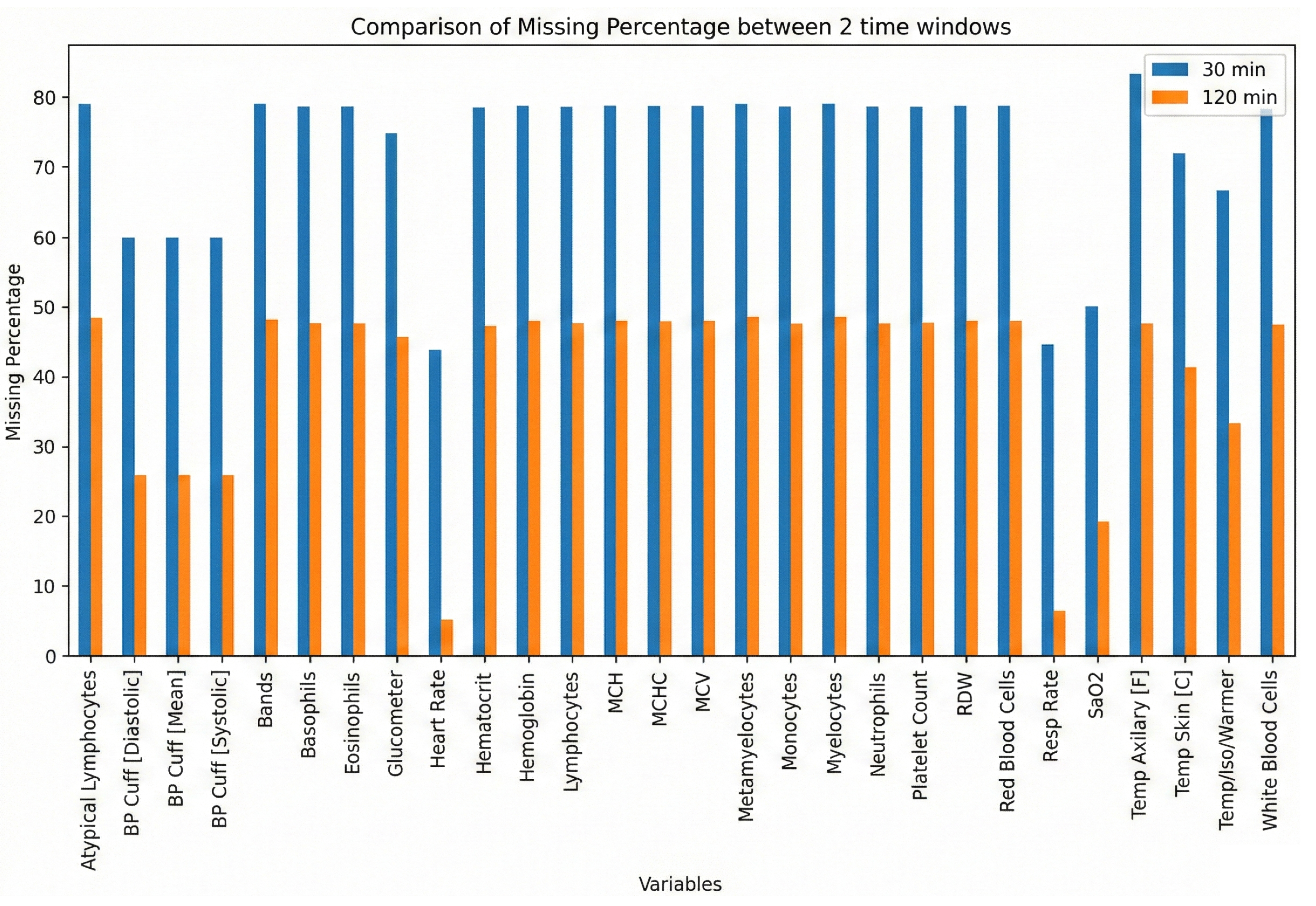
Data missing percentage of raw datasets.
We explored the nature of missingness through a multi-step approach. First, we employed missingno visualizations, which is a plot to reveal patterns of missing data in observations and variables, and a heatmap to indicate correlations in missingness [24]. Next, we performed Little’s MCAR test by label encoding categorical variables and applying mean imputation to derive a complete covariance matrix. We compared this covariance matrix to that of the fully observed subset and used the resulting statistics to ascertain whether the data were missing completely at random (MCAR). A non-significant p-value (above 0.05) supported the MCAR hypothesis, while a significant result indicated that the data might follow missing at random (MAR) or missing not at random (MNAR) mechanisms [25].
To differentiate between MAR and MNAR, we conducted chi-square tests for each variable with missing data, creating a binary indicator to evaluate associations with other observed variables; significant results suggested MAR [26]. Finally, we performed two-sample t-tests to determine if observed values differed between the “missing” and “non-missing” groups for each variable. A significant difference (p < 0.05) suggested that missingness could be MNAR, implying dependence on unobserved information rather than solely on observed data.
We examined row removal based on a pre-defined missing threshold (θ) and three imputation methods (Simple Imputer, KNN Imputer, and Iterative Imputer) for addressing missing data [27, 28]. We systematically varied θ from 0.95 to 0.6 in increments of 0.05, discarding rows that surpassed each threshold’s proportion of missing values to ensure that highly incomplete rows did not compromise imputation results. Subsequently, we artificially masked 10% of the numeric entries to create a known “ground truth” for performance evaluation, comparing original values to the imputed ones.
We used mean squared error (MSE) and mean absolute error (MAE) to assess the quality of the imputation. They were calculated over all features where masking happened. Grid search was used to adjust hyperparameters like k-values for KNN and iteration counts for the Iterative Imputer. This gave a strong benchmark for how well each method worked. This method gives a better idea of the best ways to deal with incomplete datasets by systematically measuring the trade-offs between leaving out rows and using different imputation methods.
2.5. Model Selection
We explored a diverse range of classification algorithms to capture a broad spectrum of decision boundaries, incorporating models from multiple learning paradigms, such as Linear and Statistical Models (Logistic Regression, Naïve Bayes), Tree-Based Methods (Decision Tree, Random Forest, Gradient Boosting, AdaBoost, XGBoost, LightGBM, Extra Trees, CatBoost, HistGradientBoosting, and Bagging Classifier), Instance-Based Learning (k-Nearest Neighbors), Neural Networks (Multilayer Perceptron), and Support Vector Machine [29].
This comprehensive set of models ensured that both linear and non-linear decision boundaries were considered, allowing for a more robust evaluation of classification performance.
We adopted a Stratified K-Fold cross-validation approach with five folds (n_splits = 5) for reliable assessment of model generalizability. This technique maintains consistency in class distribution across folds, mitigating potential class imbalance issues and ensuring fair evaluation across all candidate models [30].
All models’ predictive performance was assessed using the following four key metrics, computed through cross-validation:
- Accuracy: The proportion of correctly classified instances.
- Precision (weighted): The class-weighted mean of precision across all categories.
- Recall (weighted): The class-weighted means of recall, ensuring balanced sensitivity.
- F1-Score (weighted): The harmonic means of precision and recall, providing a robust measure of model effectiveness.
The mean scores for each metric were computed across all five folds, ensuring stability in performance evaluation.
The best-performing model was determined based on its mean F1-score because this metric provides a balanced evaluation of both precision and recall, making it particularly suitable for imbalanced datasets [31]. Once the top-performing model was identified, it was re-trained on the entire imputed dataset (X_imputed, y) to produce a final, optimized predictive model for validation and deployment.
2.6. Hyperparameter Optimization
We evaluated a diverse set of algorithms by employing this multi-step framework, comprising imputation, cross-validation, and metric-based model selection for the final chosen model, which exhibited strong predictive performance across multiple evaluation dimensions, enhancing its reliability for real-world applications [32].
We established a predefined grid of hyperparameter values to cover a range of model-specific configurations, such as learning rate, regularization strength, and complexity parameters. The grid systematically enumerated all possible combinations to be tested, ensuring that various configurations were explored comprehensively.
For the evaluation of each hyperparameter combination, we utilized k-fold cross-validation again. Similarly, the training data were split into k folds (e.g., k=5), and each fold in turn was treated as a temporary validation set while the remaining folds were used for model training. Five folds offered the best trade-off between statistical reliability and computation cost. Performance metrics, such as accuracy, precision, recall, or F1-score, were computed on the validation fold, and the process was repeated for each combination of parameters. This approach mitigated the risk of overfitting to a single train–validation partition and provided more robust estimates of out-of-sample performance [33].
All hyperparameter combinations in the predefined grid were iterated over, with each model built and evaluated using the cross-validation scheme described above. For Gradient Boosting, the grid spanned n_estimators (50, 100, 150), learning_rate (0.01, 0.05, 0.1), max_depth (3, 5, 7), and subsample (0.6, 0.8, 1) to balance ensemble size, step size, tree complexity, and sampling noise. For CatBoost, we varied iterations (100, 200, 300), learning_rate (0.01, 0.05, 0.1), depth (4, 6, 8), l2_leaf_reg (1, 3, 5), and border count (32, 64, 128), allowing fine-grained control over boosting rounds, tree depth, regularization strength, and stochasticity. The mean (and optionally standard deviation) of the performance metrics across folds was recorded for each parameter setting. Computational parallelization (using multiple CPU cores or threads, and the CPU is AMD Ryzen 9 3900X) was leveraged where it was feasible to expedite the search process. The configuration achieving the highest mean performance metric (e.g., the highest mean F1-score) was identified as optimal. In certain cases, a secondary performance measure (e.g., model complexity, run time) or a tiebreaker (e.g., validation loss) was used to distinguish between comparably performing solutions.
2.7. Feature Selection
The built-in feature importance mechanism of the chosen model was used to give each variable a number that showed how much it helped make predictions more accurate. We used the full feature matrix to train baseline tree-based ensembles like Random Forest, Extra Trees, Gradient Boosting, HistGradient Boosting, LightGBM, XGBoost, and CatBoost. The native importance metric for each model is the mean decrease in impurity for bagging trees and the total gain for boosting algorithms. We min-max scaled these scores to 0–1 and then averaged them to make a consensus ranking that showed which variables were considered important across models. After that, we made a ranked list of the variables, with the most important ones at the top. We then used the SHAP (SHapley Additive exPlanations) framework to figure out how much each feature added to each prediction. This gave us both summary plots and insights at the class level. This interpretability analysis helped us figure out which variables had the most significant effect on the model's predictions.
To further investigate the relationship between feature subset size and model performance, we adopted an incremental coverage scheme ranging from 10% to 80% (5% increments). Specifically, if there were F total features, a coverage level of c% dictated retaining the top [c%×F] features according to the importance ranking. For example, a coverage of 10% preserved only the top 10% of features, whereas 80% coverage retained 80% of the most important ones. At each coverage level, we trained a new CatBoost model (using the same hyperparameters) and conducted a 5-fold stratified cross-validation. The mean and standard deviation of accuracy for each subset provided insight into both performance and stability across different feature inclusion thresholds.
3. RESULT AND DISCUSSION
Table 1 presents the final list of 23 selected variables. In the 30-minute dataset, several variables exhibited notably high missingness rates (e.g., atypical lymphocytes, bands, basophils, and other hematological markers often missing in over 70% of cases), while respiratory- and temperature-related features (e.g., Heart Rate, Resp Rate, Temp Skin [C]) demonstrated comparatively lower missingness (40–70%). Overall, most mean values differed between infected and non-infected groups in the 30-minute window, with parameters like heart rate, neutrophils, and white blood cells tending to show higher average values in the infected cohort. By contrast, the 120-minute dataset contained fewer missing observations across many features (with most falling in the 20–50% range) and maintained a similar pattern of differences between infected and non-infected groups (e.g., higher heart rate, lower neutrophils among infected). Although the mean values of several variables (e.g., basophils, monocytes) remained comparable across groups, both time windows demonstrated consistent distinctions in key physiological and hematologic parameters between infected and non-infected neonates.
After conducting Little’s MCAR test, the p-value for both a 30-minute dataset and a 120-minute dataset was found to be less than 0.001, indicating that the missing data was not completely random. Then, we utilized random forest accuracy for each variable, and the result demonstrated that every row has a high accuracy (mean = 0.99).
3.1. Row Removal Threshold Result
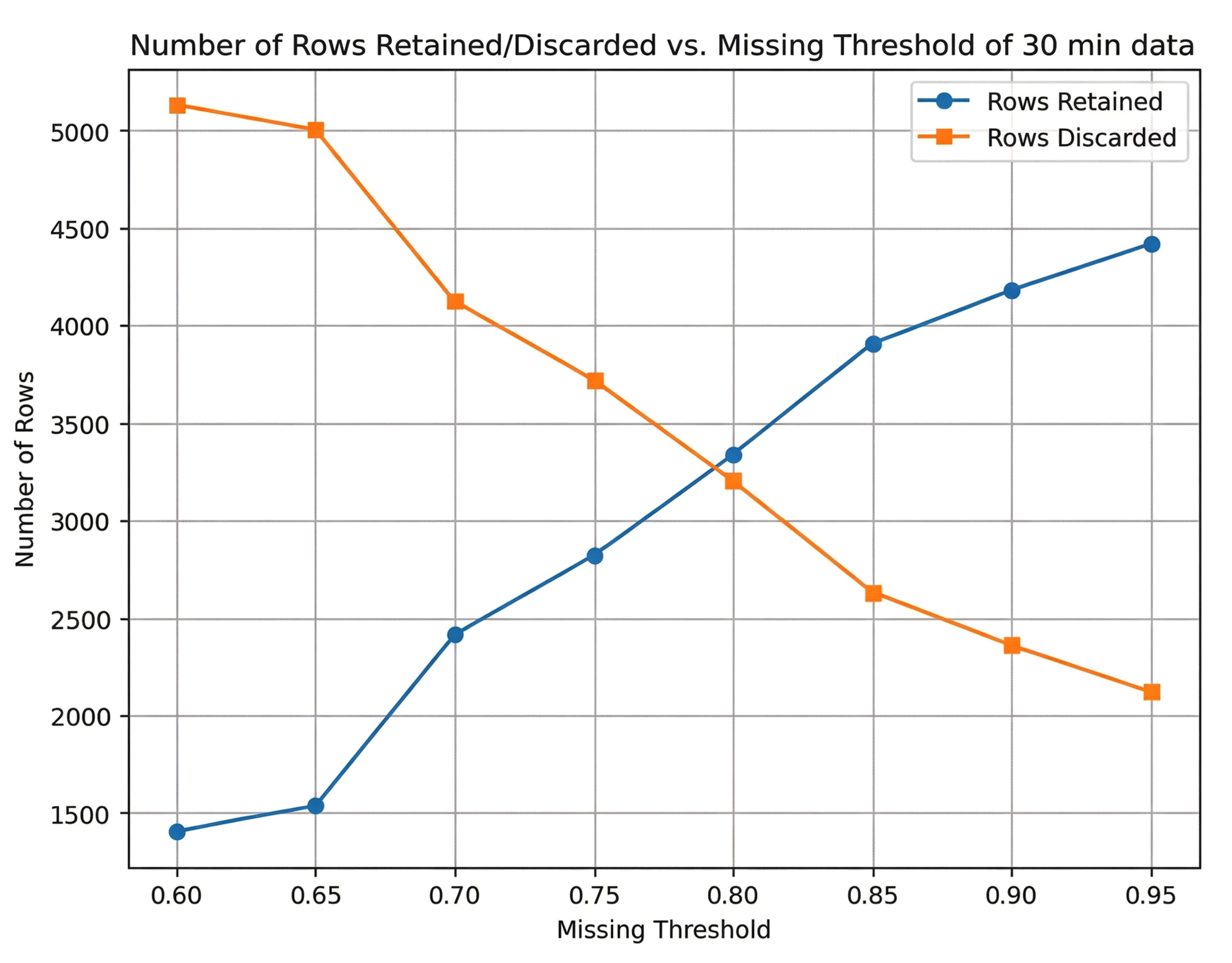
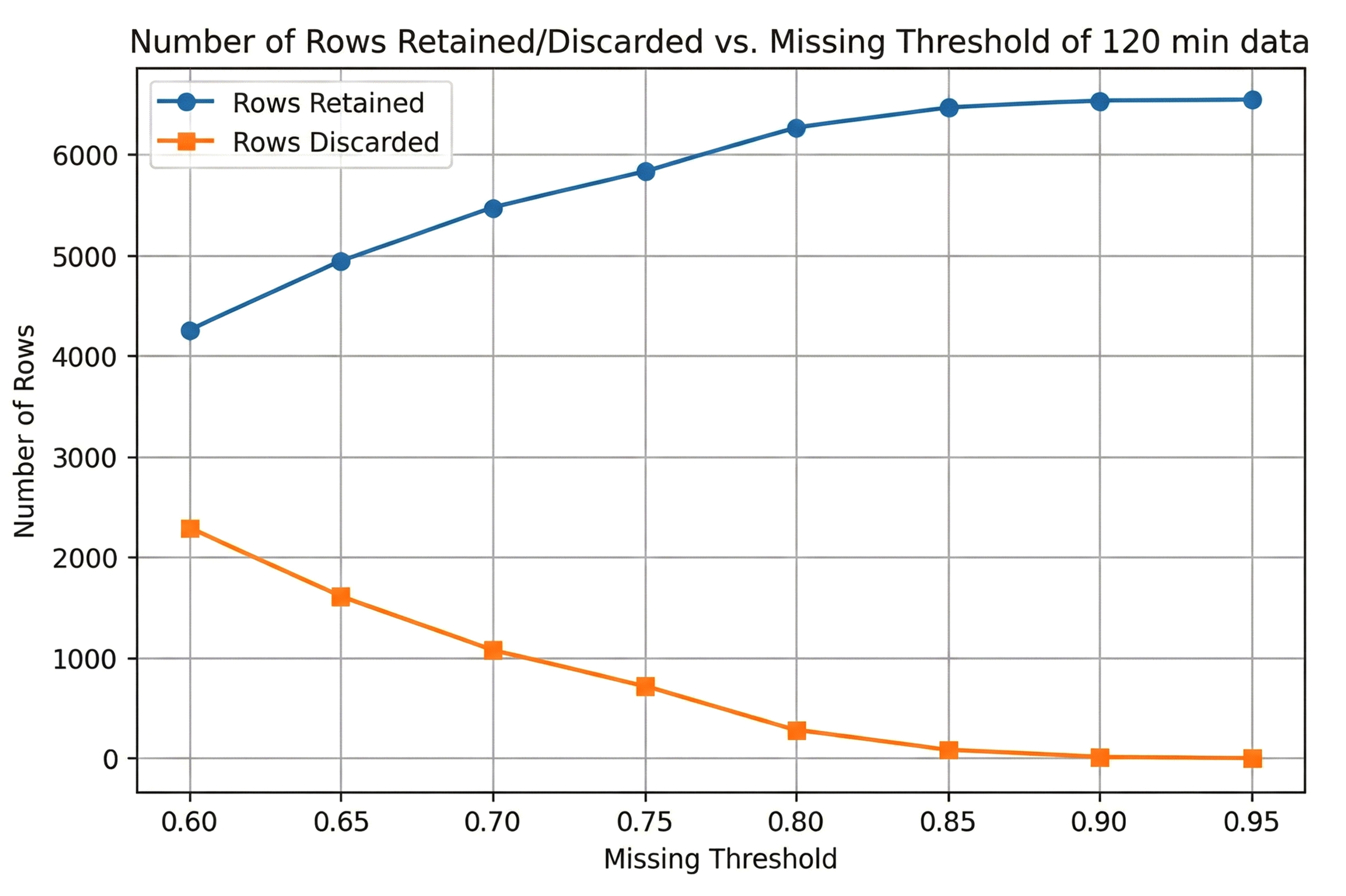
Figure 1 illustrates how varying the missingness threshold (0.60≤θ≤0.95) affects the number of retained and discarded rows for the 30-minute dataset and 120-minute dataset, respectively. As the threshold became more permissive (moving from 0.60 to 0.95), the number of retained and discarded rows changed as follows:
• 30-Minute Data: At the lowest threshold (0.60), only about 1,500 rows were retained, and around 5,000 rows were discarded, indicating that many rows exceeded 60% missingness. As the threshold increased, stricter row-removal criteria were relaxed, so more rows remained in the dataset. By a threshold of 0.95, nearly 6,500 rows were retained and fewer than 500 were excluded (Fig. 3).
• 120-Minute Data: A similar trend appeared, although even at θ=0.60, a larger portion of rows (over 4,000) was retained compared to the 30-minute dataset. This suggests that the 120-minute data had fewer high-missingness rows or more complete measurements overall. At θ=0.95, over 6,300 rows remained, and only a small fraction were removed (Fig. 4).
These results demonstrated that raising the missingness threshold substantially increased the number of retained samples, especially for the 30-minute data (which generally exhibit higher missing rates). Investigators need to find a balance between wanting to keep more data and the risk that records that are too incomplete could add noise or lower the quality of imputation.
3.2. Best Imputation Method
We systematically changed the row-removal threshold, which is the highest percentage of missing features that can be in a row, to find the best way to deal with missing data in both the 30-minute and 120-minute datasets. We then compared different imputation methods. Performance was assessed using mean squared error (MSE) and mean absolute error (MAE) relative to a “ground truth” created by artificially masking 10% of the values. For the 120-minute dataset, a threshold of 95% missingness discarded only eight rows while yielding the lowest MSE (968,311) and MAE (91.65) under Iterative Imputer (max_iter=12), demonstrating that even highly incomplete rows could be retained without severely compromising imputation accuracy. By contrast, the 30-minute data benefited from a more stringent threshold of 75%, removing 3,720 rows, to achieve the lowest MSE (962,903) and MAE (91.42) with the same imputation method. Even though the optimal thresholds differed, Iterative Imputer consistently performed better than simpler methods in both time windows. This shows how useful it is to model the relationships between variables to obtain strong imputation results.
3.3. Best Machine Learning Model
After applying the various classification algorithms to the 120-minute dataset, as shown in Fig. (5), Gradient Boosting emerged as the top performer, achieving the highest average F1-score (0.7983) across the cross-validation folds. In terms of overall classification metrics, Accuracy, Precision, Recall, and F1, Gradient Boosting consistently outperformed established ensemble methods, such as Random Forest and CatBoost, as well as linear/logistic models (e.g., Logistic Regression) and instance-based methods (KNN). This result indicates that, over a longer 120-minute window of recorded physiological and laboratory parameters, a boosted ensemble approach can successfully capture complex nonlinear patterns that distinguish infected from non-infected neonates.
Proposed approach to infection prediction in NICU of 30-minute data set.
Proposed approach to infection prediction in NICU of 120-minute data set.
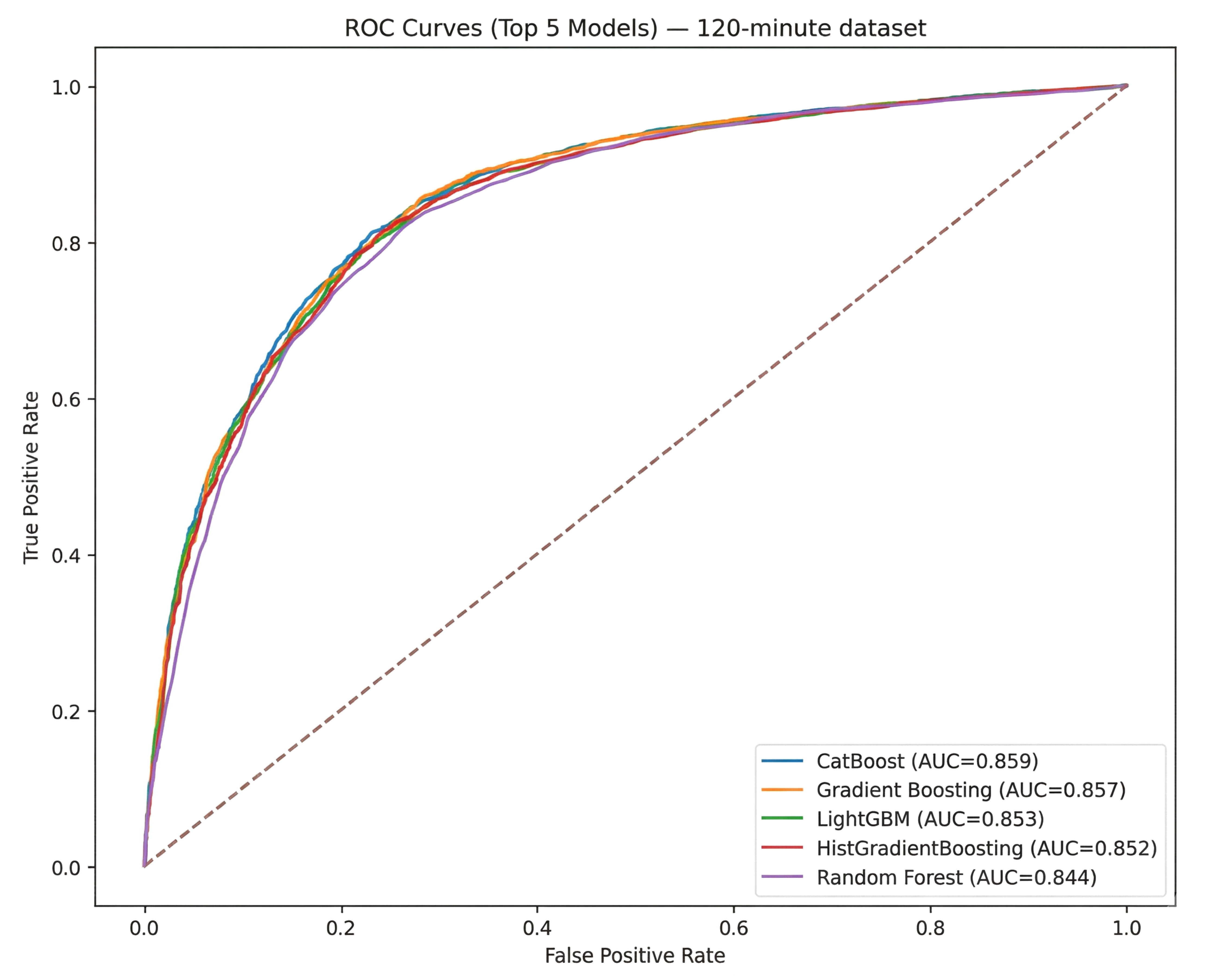
ROC for the top five models for the 120-minute dataset.
In contrast, CatBoost was found to be the best algorithm in the 30-minute data by F1-score (0.7634), narrowly surpassing Gradient Boosting (0.7628) and other tree-based methods (e.g., Random Forest, LightGBM) in terms of balanced predictive performance, as shown in Fig. (6). Although certain algorithms (e.g., Logistic Regression) also demonstrated robust Accuracy, CatBoost’s specialized handling of categorical features and iterative boosting led to more balanced gains in Precision and Recall, rendering it particularly effective in this shorter time window, where missing data and limited observation periods could constrain model inputs.
Notably, the F1-scores for Gradient Boosting (in the 120-minute data) and CatBoost (in the 30-minute data) were sufficiently close that either method could be considered a strong candidate for modeling neonatal infection risk. The next step in the experiment was to use both CatBoost and Gradient Boosting on both time windows while optimizing the hyperparameters more carefully, ensuring that the final model selection takes into account the slight differences in how each method works in different time contexts. This two-model strategy was used to figure out which boosting framework makes the most accurate and clinically useful predictions.
We conducted a grid search to optimize CatBoost and Gradient Boosting models for both the 30-minute and 120-minute datasets. Each experiment varied key parameters, such as tree depth, number of iterations (or estimators), learning rate, and subsampling rates, with cross-validation (CV) accuracy serving as the primary criterion for ranking configurations. For the 30-minute dataset, CatBoost achieved the highest CV accuracy (approximately 0.7946) under a configuration involving a moderate tree depth (depth=4) and 300 iterations at a learning rate of 0.05. By contrast, the best Gradient Boosting model on the same dataset attained a CV accuracy near 0.7903, reflecting competitive but slightly lower performance relative to CatBoost. Inspection of confusion matrices and classification reports confirmed that these top-ranked parameter sets offered balanced improvements in both Recall and Precision.
In the 120-minute setting, the situation was reversed: Gradient Boosting attained a marginally higher CV accuracy (about 0.8024) (Fig. 6), surpassing CatBoost’s best of approximately 0.8006. It was found that the optimal Gradient Boosting configuration differed from the 30-minute scenario; it favored a shallower tree (max_depth=3) with more estimators (150) and a subsampling rate of 0.8, emphasizing consistent gains in predictive performance across folds. Both models yielded robust accuracy on the fully trained dataset (ranging between 0.82 and 0.86 when evaluated via confusion matrices). However, the slight differences between the final accuracy and CV ranking indicate the importance of cross-validation for choosing hyperparameters. In particular, the alignment of strong CV scores with high out-of-sample accuracy highlights the capacity of boosted ensemble methods to capture subtle nonlinearities and interactions within newborn infection data, even under demanding early-time-window conditions.
3.4. Incremental Coverage Analysis
We performed an incremental coverage analysis where only the top-ranked features (by model-specific importance) were evaluated to assess how classification performance is influenced by the number of features retained in successive subsets. For the 30-minute dataset (using CatBoost), coverage levels ranged from 10% to 80% of the total feature set, with each subset evaluated via 10-fold cross-validation. As shown in the results table, the highest mean accuracy (0.7896) was achieved at 50% coverage, suggesting that roughly half of the most important features were sufficient to obtain robust predictive performance. Notably, while lower coverage (e.g., 10% or 25%) produced a slightly lower accuracy (0.7754 and 0.7815, respectively), including too many features at 75–80% coverage again lowered accuracy, likely due to the introduction of less informative or redundant variables (Fig. 7).
A similar procedure was applied to the 120-minute dataset with a Gradient Boosting model. It was also tested at 10% to 80% coverage. In this case, the peak accuracy (0.8058) occurred at 80% coverage, indicating that a relatively larger proportion of features contributed a meaningful signal in the extended 120-minute window. Despite a near-competitive accuracy being observed at 70% coverage (0.8045), the model benefited from retaining a broader set of features, perhaps reflecting the richer data collected over a longer timeframe. Overall, these findings underscore that an optimal balance exists between too few features (losing important signals) and too many (risking noise or redundancy). By identifying this “spot,” we can streamline model complexity while preserving high predictive performance. Table 2 presents a statistical summary of all variables across the two datasets, together with their respective missing rates.
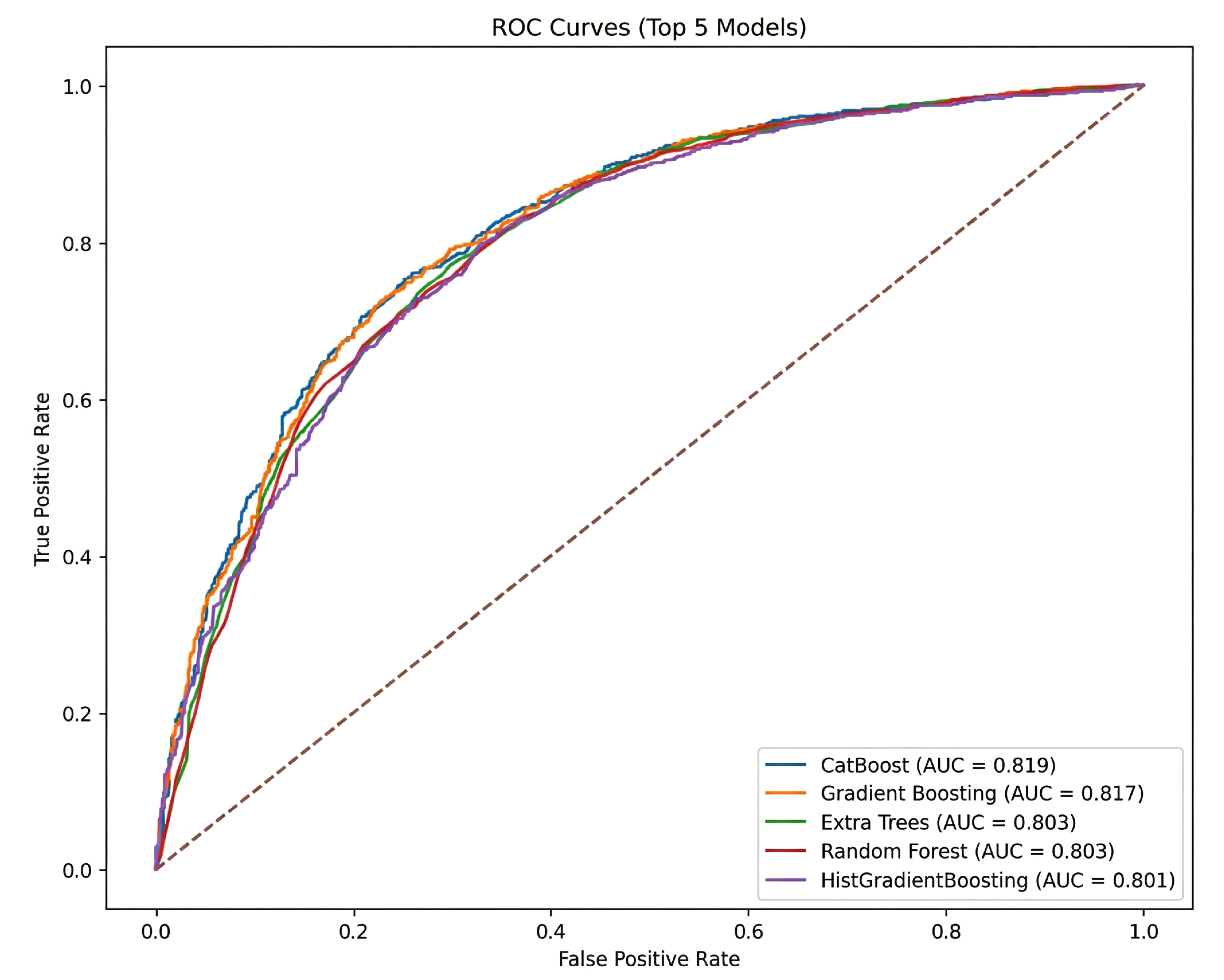
ROC for the top five models for the 30-minute dataset.
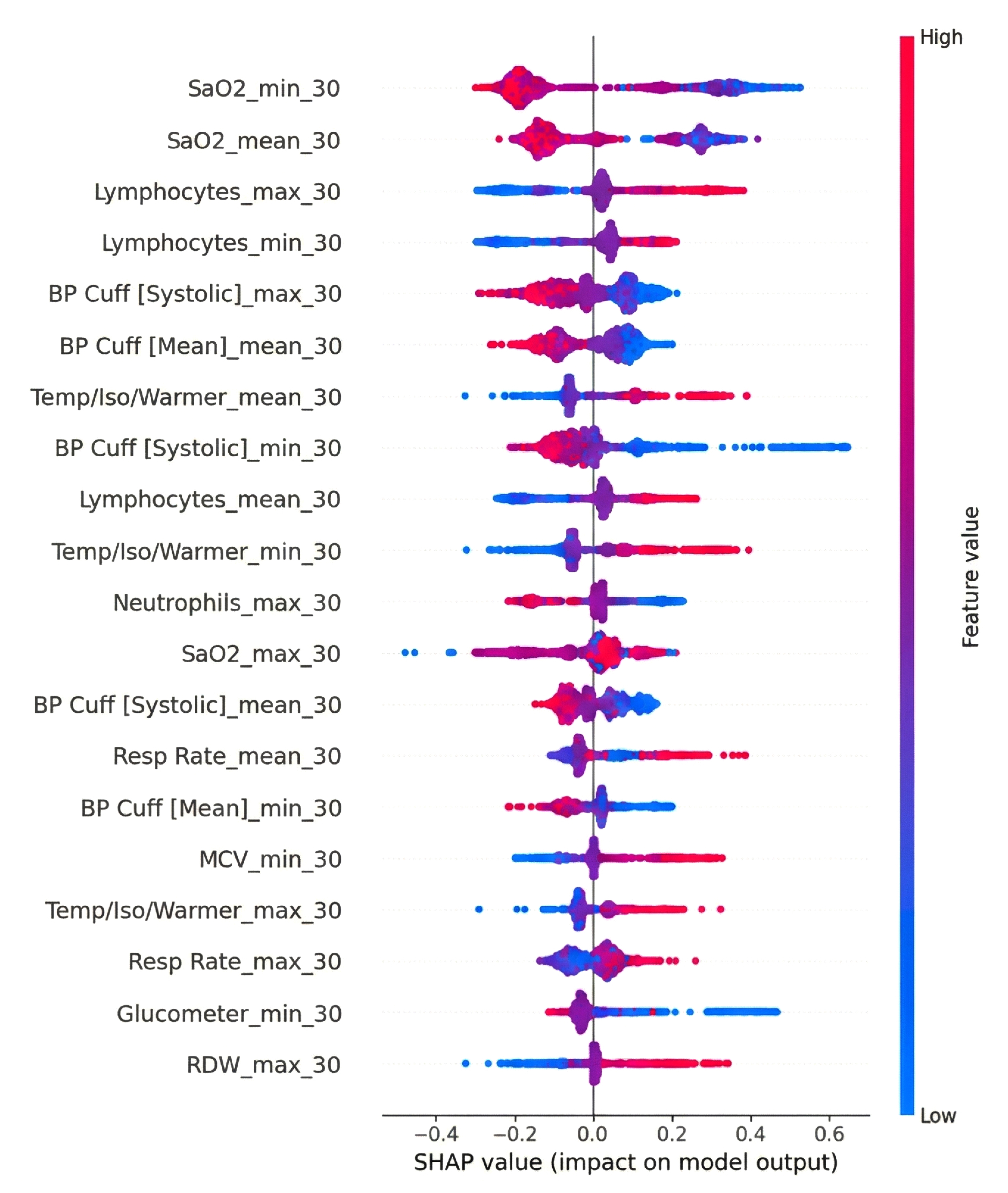
SHAP value for 30 minutes dataset of catboost.
| Variable | 30-minute Dataset | 120-minute Dataset | ||||||
|---|---|---|---|---|---|---|---|---|
| Not Infected, Mean(std) | Infected, Mean(std) | Total, Mean(std) | Missing Rate (%) | Not Infected, Mean(std) | Infected, Mean(std) | Total, Mean(std) | Missing Rate (%) | |
| Atypical Lymphocytes | 0.80 (1.64) | 1.33 (2.66) | 1.12 (2.32) | 78.84 | 0.79 (1.59) | 1.25 (2.47) | 1.03 (2.10) | 48.20 |
| BP Cuff [Diastolic] | 37.62 (8.16) | 33.60 (18.58) | 34.77 (16.35) | 59.78 | 37.64 (7.64) | 33.41 (14.89) | 34.97 (12.86) | 25.71 |
| BP Cuff [Mean] | 49.59 (8.24) | 43.75 (8.83) | 45.45 (9.06) | 59.78 | 49.77 (7.61) | 43.85 (7.80) | 46.04 (8.24) | 25.77 |
| BP Cuff [Systolic] | 68.97 (9.64) | 62.06 (16.46) | 64.07 (15.13) | 59.78 | 69.34 (8.99) | 61.99 (10.40) | 64.71 (10.52) | 25.72 |
| Bands | 2.54 (3.63) | 1.49 (3.00) | 1.91 (3.30) | 78.83 | 2.59 (3.79) | 1.72 (3.20) | 2.15 (3.52) | 48.16 |
| Basophils | 0.28 (0.60) | 0.23 (0.50) | 0.25 (0.54) | 78.54 | 0.24 (0.54) | 0.23 (0.51) | 0.24 (0.52) | 47.56 |
| Eosinophils | 2.16 (2.25) | 2.29 (2.34) | 2.24 (2.31) | 78.54 | 1.99 (1.99) | 2.24 (2.25) | 2.12 (2.13) | 47.56 |
| Glucometer | 67.60 (20.57) | 63.13 (25.64) | 64.18 (24.60) | 74.77 | 69.11 (19.12) | 69.55 (25.23) | 69.43 (23.77) | 45.70 |
| Heart Rate | 143.93 (16.58) | 149.90 (17.15) | 148.15 (17.20) | 43.71 | 141.23 (15.17) | 146.93 (15.39) | 144.83 (15.55) | 5.12 |
| Hematocrit | 51.67 (5.72) | 48.93 (6.65) | 50.04 (6.43) | 78.35 | 51.81 (5.71) | 49.03 (6.83) | 50.38 (6.46) | 47.13 |
| Hemoglobin | 17.44 (1.93) | 16.32 (2.16) | 16.78 (2.14) | 78.65 | 17.50 (1.92) | 16.38 (2.25) | 16.92 (2.17) | 47.82 |
| Lymphocytes | 30.40 (13.73) | 49.31 (19.32) | 41.69 (19.62) | 78.54 | 28.22 (12.17) | 46.79 (19.92) | 37.79 (19.03) | 47.56 |
| MCH | 35.56 (1.94) | 36.59 (2.61) | 36.17 (2.41) | 78.65 | 35.56 (1.89) | 36.74 (2.46) | 36.17 (2.28) | 47.82 |
| MCHC | 33.76 (0.94) | 33.36 (1.09) | 33.52 (1.05) | 78.67 | 33.78 (0.91) | 33.45 (1.06) | 33.61 (1.00) | 47.86 |
| MCV | 105.39 (5.27) | 109.80 (8.17) | 108.01 (7.45) | 78.67 | 105.36 (5.31) | 109.96 (7.71) | 107.72 (7.04) | 47.86 |
| Metamyelocytes | 0.25 (0.68) | 0.22 (0.78) | 0.23 (0.74) | 78.90 | 0.27 (0.70) | 0.21 (0.72) | 0.24 (0.71) | 48.47 |
| Monocytes | 6.87 (3.73) | 6.78 (3.65) | 6.82 (3.68) | 78.54 | 7.11 (3.63) | 6.91 (3.82) | 7.01 (3.73) | 47.56 |
| Myelocytes | 0.15 (0.68) | 0.12 (0.55) | 0.13 (0.60) | 78.96 | 0.14 (0.56) | 0.12 (0.52) | 0.13 (0.54) | 48.48 |
| Neutrophils | 56.59 (14.78) | 38.07 (18.80) | 45.53 (19.53) | 78.54 | 58.66 (13.49) | 40.41 (19.34) | 49.26 (19.08) | 47.56 |
| Platelet Count | 307.43 (73.73) | 275.28 (80.91) | 288.21 (79.65) | 78.64 | 301.87 (78.21) | 265.36 (81.77) | 283.00 (82.11) | 47.68 |
| RDW | 16.62 (0.97) | 17.17 (1.41) | 16.95 (1.28) | 78.68 | 16.65 (1.01) | 17.13 (1.37) | 16.90 (1.23) | 47.94 |
| Red Blood Cells | 4.92 (0.59) | 4.48 (0.71) | 4.65 (0.70) | 78.67 | 4.93 (0.57) | 4.47 (0.70) | 4.70 (0.68) | 47.86 |
| Resp Rate | 49.70 (13.33) | 51.90 (14.84) | 51.25 (14.44) | 44.55 | 48.11 (11.37) | 52.17 (12.84) | 50.66 (12.47) | 6.29 |
| SaO2 | 97.48 (5.04) | 96.00 (4.49) | 96.35 (4.67) | 49.92 | 97.85 (3.92) | 96.33 (3.16) | 96.77 (3.47) | 19.10 |
| Temp Axillary [F] | 98.41 (0.70) | 98.51 (0.83) | 98.49 (0.80) | 83.25 | 98.52 (0.61) | 98.71 (0.71) | 98.66 (0.69) | 47.51 |
| Temp Skin [C] | 36.60 (4.77) | 36.57 (3.94) | 36.57 (4.10) | 71.92 | 36.53 (3.94) | 36.58 (3.72) | 36.57 (3.77) | 41.33 |
| Temp/Iso/Warmer | 35.95 (3.02) | 36.27 (1.84) | 36.20 (2.15) | 66.63 | 35.87 (3.05) | 36.13 (2.36) | 36.06 (2.55) | 33.15 |
| White Blood Cells | 17.06 (5.57) | 13.00 (6.01) | 14.64 (6.16) | 78.42 | 17.27 (5.47) | 13.02 (6.54) | 15.08 (6.41) | 47.32 |
4. LIMITATIONS
The first limitation is data quality and heterogeneity. Although we used standardized ICU data from MIMIC-III, variations in measurement frequency, device calibration, and charting practices can introduce biases. The real-world deployment of our model, especially in other institutions, would require local calibration and external validation. In this study, we explored multiple machine learning–based methods for predicting neonatal infection risk and compared their performances with a more conventional reference scoring system. Specifically, we aimed to identify an algorithm that could accurately predict infection-related outcomes when data are aggregated either from the first 30 minutes or the first 120 minutes of intensive care unit (ICU) admission. Our findings revealed notable differences in the models’ performances across these two time windows, highlighting the trade-offs of each approach for real-world clinical use.
We only extracted variables from the first 30 or 120 minutes. Future work could incorporate dynamic, time-series features beyond these discrete windows or investigate sliding-window updates (e.g., every 15 minutes) to capture evolving physiologic patterns.
Although CatBoost and Gradient Boosting can produce feature-importance estimates or SHAP values, the underlying mechanisms remain “black box” at the bedside. Efforts to embed transparent, clinically interpretable frameworks (e.g., rule-based ensembles) might further facilitate end-user adoption.
To ensure transportability across hospital systems, future work should conduct external validation using leave-one-hospital-out and temporal designs, and, where feasible, a short prospective “shadow” deployment at new sites. Before testing, it is recommended to harmonize ontologies and units, align device and charting differences, and lock preprocessing (imputation/ standardization) on training sites only, applying it unchanged to held-out sites to prevent leakage. Moreover, it is suggested to report site-specific and pooled (random-effects) AUROC/AUPRC and calibration (intercept/slope, Brier), compare global vs. site-specific thresholds with lightweight local recalibration (intercept-only, Platt, isotonic), and when data cannot leave an institution, use privacy-preserving/federated evaluation with secure aggregation that returns only metrics and plots.
CONCLUSION
In this study, we explored multiple machine learning–based methods for predicting neonatal infection risk and compared their performances with a more conventional reference scoring system. Specifically, we aimed to identify an algorithm that could accurately predict infection-related outcomes when data are aggregated either from the first 30 minutes or the first 120 minutes of intensive care unit (ICU) admission. Our findings showed that the models worked very differently in these two time windows, highlighting the pros and cons of each method for real-world clinical use.
OVERVIEW OF FINDINGS
In the 30-minute dataset, CatBoost emerged as the top-performing model with the highest F1-score (~0.7634), surpassing Gradient Boosting (~0.7628) and other tree-based or linear methods. The marginal gap between CatBoost and Gradient Boosting suggests that, when data are relatively sparse (i.e., at only 30 minutes into an ICU stay), subtle differences in how ensemble algorithms handle missingness, outlier measurements, and imputation steps can substantially shape final performance metrics. CatBoost’s specialized handling of categorical data, alongside robust boosting iterations, may have conferred an advantage in the “ultra-early” context, where variable availability is inconsistent, and the physiologic signals can be less stable.
When the time window was extended to 120 minutes, Gradient Boosting models exhibited the highest average F1-score (~0.7983) and displayed excellent calibration. This improvement likely stems from the greater data richness at 120 minutes; additional laboratory results, updated vital signs, and time for more hemodynamic fluctuations can allow gradient-boosted ensembles to better capture complex, nonlinear relationships. Nonetheless, CatBoost, Random Forest, and certain neural network models also demonstrated strong discriminatory ability (F1-scores typically above 0.76), implying that multiple algorithmic families can achieve clinical usefulness once enough data points become available. The key difference was that Gradient Boosting reached slightly higher and more consistent cross-validation scores across accuracy, precision, and recall metrics.
INTERPRETATIONS AND CLINICAL IMPLICATIONS
Our findings highlight the significance of time-dependent data accessibility in infection-risk modeling. The 30-minute window allows to intervene very early, but it also means that the data is limited, with fewer blood gas analyses or lab results that are not completed. So, advanced methods work well with missing data or can use categorical inputs well.
The 120-minute dataset, on the other hand, provides a better overall picture of the patient's health. Taking more vital signs, conducting more lab tests, and monitoring the heart and brain for more extended periods of time can all help to make risk estimates more accurate. Gradient Boosting works better in the 120-minute window. This shows that ensemble-based methods can leverage detailed information to model more complex relationships between variables.
These results indicate a two-stage or adaptive methodology: (1) an ultra-early model appropriate for the initial 30 to 60 minutes of admission, utilizing robust management of missing data (CatBoost or a comparable boosted technique), and (2) a refined model (e.g., Gradient Boosting) re-trained with updated data at approximately 120 minutes, providing a more precise prediction for ensuing critical-care decisions.
COMPARISON WITH EXISTING LITERATURE
Several prior investigations have compared machine learning models (e.g., Random Forest, XGBoost, and neural networks) against established clinical scoring systems for sepsis or infection-related mortality. Consistent with those reports, we found that ensemble-based algorithms offer better calibration and higher F1 scores than classical logistic regression or basic scoring systems (e.g., APACHE II or simplified risk scores). Notably, the incremental gains are especially relevant in the “intermediate” time frame (1–2 hours), when important physiologic trends start to manifest yet remain absent at baseline.
AUTHORS’ CONTRIBUTIONS
The authors confirm contribution to the paper as follows: Z.C. and Z.Q.: Study conception and design; Z.C.: Data collection; Z.C.: Analysis and interpretation of results; Z.C.: Draft manuscript. All authors reviewed the results and approved the final version of the manuscript.
LIST OF ABBREVIATIONS
| ICU | = Intensive Care Unit |
| NICU | = Neonatal Intensive Care Unit |
| ML | = Machine Learning |
| SHAP | = SHapley Additive exPlanations |
| MIMIC-III | = Medical Information Mart for Intensive Care III |
| MCAR | = Missing Completely at Random |
| MAR | = Missing at Random |
| MNAR | = Missing Not at Random |
ETHICS APPROVAL AND CONSENT TO PARTICIPATE
The creation and sharing of MIMIC-III were approved by the Institutional Review Boards of Beth Israel Deaconess Medical Center (BIDMC, Boston, MA, USA; Protocol 2001-P-001699/14) and the Massachusetts Institute of Technology (MIT COUHES, Cambridge, MA, USA; Protocol 0403000206), with a waiver of informed consent.
HUMAN AND ANIMAL RIGHTS
All procedures performed in studies involving human participants were in accordance with the ethical standards of institutional and/or research committee and with the 1975 Declaration of Helsinki, as revised in 2013.
CONSENT FOR PUBLICATION
The MIMIC-III database contains only de-identified data, and the BIDMC and MIT IRBs granted a waiver of informed consent for the database’s creation and sharing; no identifiable patient information or images are published in this manuscript.
AVAILABILITY OF DATA AND MATERIALS
The datasets analyzed during the current study are publicly available in the MIMIC-III Clinical Database (v1.4), hosted by the Massachusetts Institute of Technology (MIT) Laboratory for Computational Physiology. Access is granted to qualified researchers after completion of the required data use agreement and training.
ACKNOWLEDGEMENTS
The authors would like to thank the MIT Laboratory for Computational Physiology and Beth Israel Deaconess Medical Center for maintaining and providing access to the MIMIC-III database. They would also like to thank colleagues from the Department of Biostatistics and Bioinformatics at Emory University for their valuable discussions and feedback during the preparation of this study.