Detection of Dementia: Using Electroencephalography and Machine Learning
Authors Info & Affiliations
Abstract
Introduction
This article serves as a background to an emerging field and aims to investigate the use of Electroencephalography signals in detecting dementia. It offers a promising approach for individuals with dementia, as electroencephalography provides a non-invasive measure of brain activity during language tasks.
Methods
The methodological core of this study involves implementing various electroencephalography feature extraction and selection techniques, along with the use of machine learning algorithms for analyzing the signals to identify patterns indicative of dementia. In terms of results, our analysis showed that most individuals likely to have dementia are in the 60-69 age bracket, with a higher incidence in females.
Result
Notably, the K-means algorithm achieved the highest Silhouette Score at approximately 0.295. Additionally, Decision Tree and Random Forest models achieved the best accuracy at 95.83%, slightly outperforming the support vector machines and Logistic Regression models, which also showed good accuracy at 91.67%.
Conclusion
The conclusion drawn from this article is that electroencephalography signals, analyzed with machine learning algorithms, can be effectively used to detect dementia, with Decision Tree and Random Forest models showing promise for future non-invasive diagnostic tools.
1. INTRODUCTION
A collection of symptoms that significantly impair thinking, memory, and social skills to the point that they interfere with day-to-day functioning is referred to as dementia. It is most typically caused by Alzheimer's disease, which affects and eventually destroys brain cells [1]. It is frequently, but not always, a hallmark of aging. Infections, head trauma, strokes, and other illnesses, including Parkinson's or Huntington's disease, can also result in dementia symptoms [2]. Dementia can cause mood swings, personality changes, disorientation, memory loss, and communication difficulties. It is anticipated that the number of dementia cases would rise sharply in the upcoming years, with 152 million people worldwide predicted to have dementia by 2050 [3]. Therefore, there is a pressing need to develop effective methods for the early detection and treatment of dementia.
The term “EEG” (electroencephalography) describes the methods and software used to examine and decipher the electrical signals that the brain produces and processes, as captured by EEG sensors. The raw EEG signals may be processed to obtain useful properties, including frequency, amplitude, and power [4]. These signals provide information about brain activity. The analysis of EEG signals can yield important information about how the brain works and aid in the identification of diseases, including dementia, epilepsy, sleep problems, and brain traumas.
Analyzing and interpreting EEG data using machine learning yields promising results [5]. Machine learning algorithms may be trained to identify patterns in EEG data, which represent the electrical activity of the brain, in order to monitor brain function, diagnose neurological disorders, and make predictions.
EEG uses a range of machine learning techniques [6], such as deep learning algorithms like Convolutional Neural Networks (CNNs) and Recurrent Neural Networks (RNNs), clustering algorithms like k-means and hierarchical clustering, and classification algorithms like support vector machines (SVMs) and decision trees. Large datasets of EEG signals may be used to train these algorithms to identify patterns that correspond to various brain conditions or states.
Brain-computer connections, seizure detection, and sleep stage classification are just a few of the many uses for EEG machine learning [7]. Because it offers a non-invasive and effective method of analyzing vast volumes of EEG data, it has the potential to completely change how we diagnose, treat, and monitor neurological diseases as well as how we monitor brain activity.
1.1. Types of Dementia
A range of cognitive illnesses that are characterized by a loss in thinking, reasoning, and memory that interferes with day-to-day functioning are collectively referred to as dementia. Brain cell damage that impairs the brain's capacity to communicate and function normally is the cause of dementia. Depending on the form of dementia, many reasons may apply. These are a few prevalent forms of dementia, along with their causes:
i. Alzheimer's Disease: It is estimated that between 60 and 80 percent of dementia cases are caused by Alzheimer's disease. It is typified by the buildup of aberrant protein deposits in the brain, such as tau tangles and amyloid plaques, which eventually cause the loss of brain tissue and function [8]. Alzheimer's disease symptoms include confusion about time and location, memory loss, and difficulty solving issues. Although the precise origin of Alzheimer's disease is unknown, age-related changes in the brain, genetics, and lifestyle choices are thought to be involved.
Current tools to diagnose Alzheimer's dementia using AI algorithms can analyze brain MRI or PET scans to detect specific patterns and biomarkers. For instance, CNNs can identify abnormal brain structures indicative of Alzheimer's disease or Lewy body dementia.
ii. Vascular Dementia: The second most prevalent kind of dementia is vascular dementia, which is brought on by decreased blood supply to the brain, which damages the parts of the brain involved in cognitive processes. Decision-making issues, poor judgment, and diminished decision-making capacity are among the signs and symptoms of vascular dementia [9].
ML models that can analyze cognitive assessment data, such as neuropsychological tests, to find patterns of cognitive deterioration are now used as diagnostic tools for vascular dementia. For example, temporal changes can be detected by LSTM networks through analysis of longitudinal cognitive data.
iii. Lewy Body Dementia (LBD): The brain's aberrant protein deposits known as Lewy bodies are what define Lewy body dementia. These deposits cause symptoms related to cognition and motor function in the brain. Movement issues, vivid nightmares, and visual hallucinations are signs of Lewy Body Dementia [10].
AI may be used to develop individualized treatment plans and assist in the early diagnosis of Lewy Body Dementia by identifying possible biomarkers, such as genetic markers or protein levels in blood or cerebrospinal fluid, that may indicate a particular kind of dementia.
iv. Frontotemporal Dementia (FTD): The gradual degradation of nerve cells in the brain's frontal and temporal lobes is the cause of frontotemporal dementia. Frontotemporal dementia is a condition that primarily affects younger people and impairs behavior, demeanor, and language difficulties [11].
NLP techniques are used to examine voice data's linguistic content and identify changes in language usage and grammar linked to frontotemporal dementia (FTD). This is one of the current methods for diagnosing frontotemporal dementia. Multimodal fusion approaches may be used to combine speech and EEG data, improving the diagnostic accuracy of FTD detection models.
This manuscript is restricted to Alzheimer's disease. Effective management and treatment of dementia need early diagnosis and proper medical attention.
1.2. Aim of The Study
This research proposes a methodological solution (PMS) that involves advanced feature extraction techniques and addresses the following key operational research questions (ORQ) given below:
1. Put into practice and validate a set of machine learning models to improve the precision of EEG-based dementia diagnosis greatly.
2. The quality of the EEG data is significantly improved for dementia diagnosis by evaluated preprocessing procedures, including filtering, denoising, and artifact removal.
3. Examined several machine learning techniques, including DT, SVM, RF, and K Means, and determined which patterns and clusters in the EEG data were the most efficient and distinctive.
4. Machine learning models for dementia detection that have been examined work well for people of different ages and genders, laying the groundwork for more individualized diagnosis.
This research study is structured as follows. As stated in Section 1, the introduction is covered in Section 2, along with associated work, methodology, data preprocessing, and feature engineering in Section 3, results and discussion in Section 4, and conclusion and prospects in Section 5.
2. RELATED WORK
The non-invasive technique of electroencephalography (EEG) has been used to identify anomalies in brain activity linked to dementia. The use of EEG to assist in the diagnosis of dementia, including Alzheimer's disease (AD) and other types of dementia, has been investigated in a number of studies. The earliest and most important investigation using EEG as a tool for early AD identification was conducted by Jelles et al. in [12]. The results of the study showed that EEG spectrum analysis could distinguish between individuals with dementia and healthy controls, indicating that EEG may be a valuable diagnostic tool for dementia early detection. Another study conducted in [13] by Jeong et al. investigated the use of EEG to differentiate between AD, vascular dementia, and dementia with Lewy bodies. According to the study, EEG has a high degree of accuracy in differentiating between these dementia forms, indicating that it may be a valuable tool for dementia differential diagnosis. Later in the year, Babiloni et al. [14] also provided an overview of the state of the research on EEG as a dementia diagnostic tool. According to the research, EEG abnormalities were consistently seen in dementia patients, and the test may distinguish between various forms of dementia. The study did point out that further research is required to determine the clinical relevance of EEG for dementia diagnosis, as it has limits in terms of sensitivity and specificity.
Subsequent research has examined the processing of EEG waves using machine learning approaches to identify dementia. EEG data have been used to train machine learning algorithms for a range of tasks, such as the categorization of EEG patterns, the prediction of mental states, and the identification of neurological illnesses. EEG data, for instance, have been used to detect neurological conditions like epilepsy and schizophrenia, predict cognitive states like attention and memory, and categorize various sleep stages [15].
Support vector machines (SVMs) are one of the most used machine learning techniques for EEG analysis. It has been demonstrated that SVMs are useful for identifying neurological illnesses and categorizing EEG patterns. SVMs, for instance, were employed to categorize EEG data in research by Zhang et al. [16], with a sensitivity of 86.67% and specificity of 91.11% [17]. Decision trees are another well-liked machine learning approach for EEG analysis. These algorithms have been used to identify different mental states and evaluate EEG data. For instance, decision trees were utilized in research by Feng et al. in [18] to identify EEG signals, and the results showed a sensitivity of 85.71% and specificity of 89.47% [18].
Convolutional neural networks (CNNs) and recurrent neural networks (RNNs), two deep learning techniques, have been used on EEG data more recently. It has been demonstrated that deep learning algorithms are useful for identifying different mental states and neurological conditions as well as for categorizing EEG patterns. For instance, a deep neural network was employed in a study by Liu et al. [19] to classify EEG data with an accuracy of 87.5%.
An investigation on the use of EEG power spectra as a possible biomarker for Alzheimer's disease diagnosis was carried out by Lopez-Sanz et al. in [20]. They gathered EEG data from both healthy controls and Alzheimer's patients, and they examined the power spectra across several frequency ranges. The power spectra of the two groups differed significantly, according to their findings, with Alzheimer's patients showing lower power in particular frequency bands. They came to the conclusion that EEG power spectra could be a helpful biomarker for early detection of Alzheimer's disease.
In order to determine if electroencephalography (EEG) may be utilized as a biomarker for cognitive impairment in this group, Gómez et al. evaluated the use of EEG in older persons in research published in [19]. They examined EEG signals from an elderly population, comprising those with slight cognitive impairment and those without it. Their total accuracy using SVM and four EEG frequency bands was 74.2%.
In summary, the crucial preprocessing step of removing artifacts from the data has not received enough attention in the present study on dementia diagnosis utilizing EEG signals and machine learning. This discrepancy may cause errors and lower the accuracy of detecting techniques. For the accurate diagnosis of dementia, the quality of the EEG data is essential. One significant gap that impacts the efficacy of machine learning algorithms in accurately diagnosing dementia is the absence of thorough data preparation, particularly the removal of artifacts and filtering in previous studies.
3. METHODS
The suggested research pipeline is depicted in Fig. (1) and consists of data preprocessing, feature engineering, and machine learning. These steps must be carefully planned and executed to guarantee that the dataset is balanced and does not overrepresent any one form of dementia or severity level. The objective is to create a clean, accurate, and representative dataset of the various forms of dementia so that machine learning algorithms can offer trustworthy, objective diagnoses and insights. By using EEG signals, our suggested technique improves the accuracy and reliability of dementia detection.
3.1. Data Collection
In this work, we have employed the Open-Neuro dataset, which is accessible to the public [21]. The EEG data from 88 patients in total are included in this dataset; 44 of the subjects are male, and 44 are females, with a mean age of 66.52 for men and 65.82 for women [21].
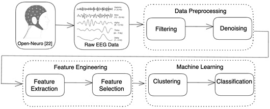
Proposed methodology.
An electroencephalograph [22] is one piece of specialist equipment that may be used to capture EEG data. Afterwards, the signals are processed and analyzed using a variety of software tools in order to identify patterns that can be suggestive of dementia or cognitive decline. In certain situations, the patient may be asked to sit quietly with their eyes closed or open while in the resting state, or the EEG data may be obtained while the patient is doing a particular cognitive activity, such as an attention or memory test. To get precise and trustworthy EEG data, it's critical to make sure the patient feels at ease and content during the recording. The International 10-20 System Electrode Placement Method is the approach that is most frequently used to get EEG data.
One popular technique for placing electrodes on the scalp during electroencephalography (EEG) recording is the international 10-20 system. It is a systematic procedure that guarantees uniform and precise electrode insertion in various people, which is essential for analyzing and interpreting EEG signals.
The term “10-20” describes the separations between neighboring electrode placements, which are 10% and 20%, respectively, of the whole front-back and right-left lengths of the scalp. Based on the structure of the brain, this approach separates the scalp into several areas, and each electrode implantation is labeled with a letter and number to designate its position [22].
Fig. (2) [22] illustrates the various locations of the brain's lobes. The distance from the midline is indicated by the number (even numbers for the right side and odd numbers for the left), which also tells which lobe of the brain the area is closest to. The sculp data has been specified using the electrode montage selector. The letters Frontal (F), Central (C), Parietal (P), Occipital (O), and Temporal (T) represent the five primary sculps [22].
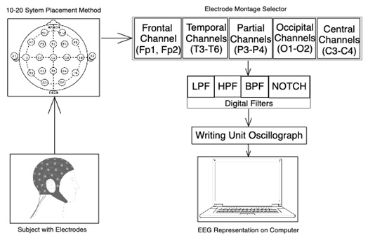
International 10-20 system electrode placement method [22].
In addition, drift or electrode offset has been eliminated using an LPF with a 30-Hz cutoff and an HPF with a 1-Hz cutoff. These filters have a 60-120 second time frame and are fed into a writing unit oscillograph to produce EEG signals that are sent to a PC.
3.2. Data Preprocessing
The collected EEG data is preprocessed using MATLAB SIMULINK [23] to reduce noise filtering and artifacts from EEG signals through a variety of techniques, such as filtering, artifact removal, and denoising algorithms explained below:
3.2.1. Noise Filtering
EEG signals may be cleaned up from undesired noise by using a filtering approach [24]. To exclude particular noise frequencies from a signal, one may design and apply a variety of filters in MATLAB SIMULINK, including band-pass, low-pass, high-pass, and notch filters. We have used band-pass filters for this activity so that we only keep the frequencies that are relevant (usually between 1 and 40 Hz for most cognitive activities). As shown in Fig. (3), This will help eliminate any high-frequency noise as well as very low-frequency drifts to avoid distorting the time relationships within the signal. This can be particularly important in cognitive tasks where timing information is crucial. The criteria for this bandpass filter design were to provide a smooth response in the passband and a relatively flat frequency response, which minimizes distortion because it has no ripple in the passband and doesn't attenuate as rapidly as other types.
3.2.2. Artifact Removal
Many causes, including electrode movement, muscular activity, and eye movement, can result in artifacts in EEG signals [25]. To eliminate artifacts from the signal, MATLAB SIMULINK offers a number of artifact reduction algorithms. Fig. (3) illustrates this, particularly in frontal channels like Fp1 and Fp2, which are frequently impacted by artifacts connected to the eyes.
MATLAB SIMULINK offers a variety of denoising methods that may be used to eliminate noise from EEG recordings. The wavelet denoising technique has been utilised to divide the signal into distinct frequency bands and eliminate noise from each band independently [26].
In order to eliminate certain frequency noise, we have also employed notch filters for this objective. Notch filters are made to eliminate or greatly reduce frequencies within a very precise range. This is perfect for removing some kinds of interference, such as powerline noise, which frequently causes issues with EEG recordings. Depending on the area, powerline noise normally occurs at 50 Hz or 60 Hz. A notch filter may precisely target these frequencies.
Notch filters have little effect on frequencies outside of their narrow stopband, in contrast to band-pass or low-pass filters, which affect a wider range of frequencies. This is significant for EEG analysis since accurate interpretation depends on maintaining the signal integrity throughout a range of frequency bands.
Fig. (4) shows the decomposed signal into wavelet coefficients, then thresholds these coefficients to remove noise, and finally reconstructs the signal from the denoised coefficients.
By applying filters consistently across all channels, it becomes easier to identify and address these artifacts, as their impact on the signal will be uniform.
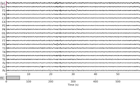
Noise filtering using band-pass filter.
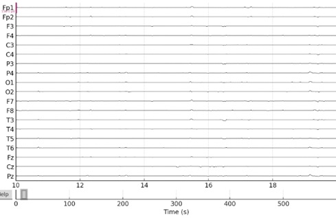
Signals after artifact removal using notch filters.
3.3. Feature Engineering
Creating machine learning models requires a crucial stage called feature engineering. It entails producing, selecting, and converting unprocessed data into characteristics that improve the efficiency of machine learning systems. It basically involves transforming unprocessed data into a format that is more appropriate for modeling. Feature extraction and feature selection, which are covered below, are two possible steps in this procedure.
3.3.1. Feature Extraction
By converting the original features into a new set with less redundancy and more discriminating power, feature extraction is a machine-learning approach that reduces the dimensionality of a dataset. The following are some methods for lowering a dataset's dimensionality via feature extraction:
3.3.1.1. Independent Component Analysis (ICA)
ICA is a technique used for feature extraction that aims to separate a set of signals into their underlying independent sources [24]. The original features are transformed into a new set of features that represent the independent sources, which can have reduced dimensionality compared to the original data.
The weight or contribution of each EEG channel to the independent component is represented by the spatial topographies. The data are divided into statistically independent components using ICA. These elements frequently stand in for different neuronal or non-neural activity sources.
The color scales in Fig. (5) depict the relative importance or weight of every EEG channel. The ICA's components aren't always arranged according to variance, though. Rather, there is no statistical difference between them. Because ICA can distinguish between brain activity and noise sources like muscular contractions or eye blinks, it is very helpful in identifying and eliminating artifacts. Certain components, including heartbeats or eye blinks (which are frequently observed as frontal activity on channels like Fp1 and Fp2), may mimic common EEG artifacts.
3.3.1.2. Principal Component Analysis (PCA)
PCA is a common technique used for feature extraction in which the original features are transformed into a new set of orthogonal features that capture the most important information in the data [18]. The new features are ordered in terms of their importance, so the first few principal components can be used to represent the data with reduced dimensionality.
The loading or weight of each EEG channel in the corresponding PCA component is represented by the spatial topographies. These components show the directions in which the data fluctuates the greatest and are orthogonal to one another.
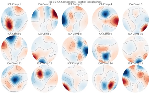
Weight of each EEG channel using ICA.
The direction with the largest variance is represented by the first component (PCA Comp 1) in Fig. (6), the direction with the second maximum variance (orthogonal to the first) by the second component (PCA Comp 2), and so on. The color scales show each EEG channel's weight or loading. For example, negative weights are represented by dark blue or purple, whereas positive weights are represented by yellow or red. The way that each component condenses various elements of the EEG data is reflected in these spatial patterns. Some components might capture widespread activity across many channels, while others might emphasize localized activity in specific regions.
Therefore, PCA works well to reduce the number of dimensions in the data while preserving the majority of the variance. This is important when using EEG analysis to identify dementia, as the data from many electrodes might be high-dimensional, and the most important information may be captured by a small number of main components. Furthermore, PCA is a simple and computationally effective approach. It is simpler to use and faster to compute since it does not involve sophisticated computations like ICA, LDA, and ITA or assumptions about the distribution of the data.
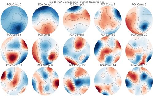
Weight of each eeg channel using PCA.
3.3.2. Feature Selection
The process of choosing a subset of pertinent characteristics from a broader set of features is known as feature selection, and it aids in lowering the dataset's dimensionality [26]. We may enhance the efficiency of machine learning algorithms, lower computing complexity, and avoid overfitting by minimizing the number of features. The following are some typical methods for choosing features:
3.3.2.1. Filter Method
Statistical measurements are used in the filter approach to rank the features and choose the best characteristics. As an illustration, consider feature selection techniques like chi-square, mutual information, and correlation-based feature selection [27].
The top EEG channels are shown in Fig. (7), utilizing the filter approach for feature selection, depending on their connection with variance. The top EEG channels are shown on the y-axis. Additionally, each channel's association with the variation between time points is shown on the x-axis. The total variation in the EEG data is more strongly correlated with channels that are closer to the left (with more negative values) or the right (with more positive values). As an example, the channels “Fp1” and “Fp2” have the largest negative correlations with variance, suggesting that they account for a considerable amount of the data's unpredictability.
3.3.2.2. Wrapper Method
The wrapper technique assesses the subset of characteristics using a machine learning model. The optimal subset of features is selected after the algorithm has been trained and evaluated using various feature subsets. One illustration of a wrapper technique is recursive feature removal.
Using the Wrapper Method, Fig. (8) visualizes the top EEG channels according to their Recursive Feature Elimination (RFE) ranking. The top EEG channels are shown on the y-axis. The RFE rating is shown on the x-axis. When it comes to forecasting the target, in this example, the mean of each sample is a lower rank, which denotes greater relevance. When using a linear regression estimator in the RFE approach, channels toward the top of the plot (with lower ranking values) are considered to be more significant.
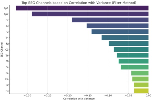
Feature selection using filter method.
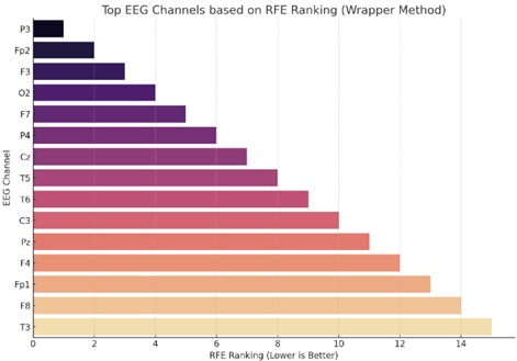
Feature selection using wrapper method.
3.3.2.3. Embedded Method
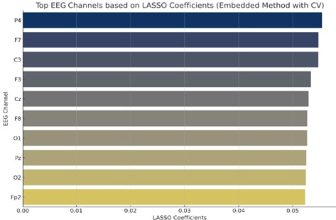
Feature selection is a step in the model training process using the embedded approach. For instance, Lasso regression adds a penalty term to the model's cost function to promote sparsity in the model's feature weights, or decision trees, where the model coefficients directly correlate to the importance of the features.
The top EEG channels are visualized using the Embedded Method with cross-validation, as shown in Fig. (9), based on their LASSO coefficients. Top EEG channels are shown on the y-axis. To illustrate the LASSO coefficients, the x-axis is used. In terms of target prediction, channels with higher coefficients—positive or negative—are seen to be more significant. The largest coefficients in this graphic correspond to channels like “P4”, “F7,” and “C3,” demonstrating their relative relevance in the model.
Feature selection using embedded method.
Clustering graphs comparison.
4. RESULTS AND DISCUSSION
4.1. Clustering
To start, we created a few groupings using clustering on the prepossessed EEG data. After that, labels are applied to these clusters for supervised learning. This method is predicated on the idea that the EEG data contains discrete, groupable patterns. There are now just 12 main components left in the data, down from 171 characteristics, after PCA was used to preserve 95% of the variance. Next, we used the K-means technique for unsupervised clustering. As our labels were binary and artificial, we will attempt to cluster the data into two clusters for simplicity's sake.
The K-means clustering algorithm has grouped the segments into two clusters:
- Cluster 0: Contains 39 segments.
- Cluster 1: Contains 80 segments.
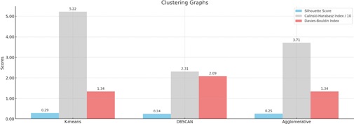
The clustering findings that were assessed using the Davies-Bouldin Index, Calinski-Harabasz Index, and Silhouette Score—an internal cluster validation measure—are displayed in Table 1 and Fig. (10). Using the following techniques, the Silhouette Score runs from -1 to 1, with a high value indicating that the item is well matched to its cluster and poorly matched to nearby clusters:
| Algorithm | Silhouette Score | Calinski-Harabasz Index | Daives-Bouldin Index |
|---|---|---|---|
| K-Means | 0.29 | 52.21 | 1.34 |
| DBSCAN | 0.24 | 23.15 | 2.09 |
| Agglomerative | 0.25 | 37.06 | 1.34 |
For each algorithm, we evaluated the clusters using the following metrics:
(a) Silhouette Score: Compared to the other algorithms, K-means produced the greatest score, indicating that its clusters had greater cohesiveness and separation. For our clustering findings, the Silhouette Score is around 0.29. The range of the Silhouette Score is -1 to 1. A score around -1 suggests that the clusters overlap, while a score near 1 shows that the clusters are well separated from one another. A score of almost 0 indicates clusters that overlap, with samples located quite near the adjoining clusters' decision borders. Our result of 0.29 indicates that there appears to be some differentiation between the two groups. Given the artificial nature of the labels and the heuristic-based methodology we employed, this is to be expected.
(b) Calinski-Harabasz Index: It is sometimes referred to as the Variance Ratio Criterion, which calculates the ratio of the total dispersion between clusters to the dispersion within clusters. Better clustering is indicated by higher values. Once more, K-means produced the best results, showing that the clusters it generated had a greater variance ratio across and within clusters.
(c) Davies-Bouldin Index: Calculates the average resemblance between each cluster and the cluster that is most like it. Better clustering is indicated by lower values. While DBSCAN has a lower score, K-means and agglomerative clustering have similar ratings.
4.2. Time-Based Segmentation & Synthetic Label Creation
We have divided the EEG data into fixed-length windows using clustering. A segment length of five seconds was our choice. This translates to 2500 samples per segment at the 500 Hz sampling rate. The EEG data was then split up into these pieces. We removed the final few samples that didn't fit into a whole segment if the EEG data didn't split precisely into these segments. Later, we determined each segment's mean amplitude. Next, using this mean amplitude as our basis, we generated a binary label: We designated a segment as “1” if its mean amplitude exceeded a threshold, with zero serving as the threshold. If not, we assigned it a value of '0'.
This method produced a binary classification issue, where segments below the threshold were labeled as “negative” (label = 0) and those with a mean amplitude above the threshold as “positive” (label = 1).
It is critical to remember that the mean amplitude heuristic was used to construct these labels, which are entirely synthetic.
The classification results are displayed in Table 2 and Fig. (11), with the Random Forest and Decision Tree models outperforming all others in terms of all criteria. While the Random Forest and Decision Tree models somewhat outperformed the SVM and Logistic Regression models, both models produced good results.
4.3. Comparison of Different Demographic Groups
The X-axis (Age) in (Figs. 12 and 13) displays the participants' ages. Plotted along this axis is the age range found in the dataset. On the other hand, the Y-axis (Number of Participants) shows how many people are involved in each age group. Participants who are “Likely No Dementia” (based on MMSE scores between 24 and 30) are shown in pink. Moreover, those with “Likely Dementia” (defined as MMSE scores between 0 and 17) are shown in the blue.
| Classifiers | Accuracy | Precision | Recall | F1 Score |
|---|---|---|---|---|
| Decision Trees | 95.83% | 95.65% | 100% | 97.87% |
| Random Forest | 95.83% | 95.65% | 100% | 97.78% |
| SVM | 91.67% | 91.67% | 100% | 95.65% |
| Logistic Regression | 87.50% | 91.30% | 95.45% | 93.33% |
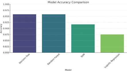
Classification graph comparison.
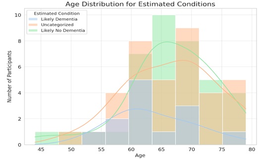
Dementia prediction by age.
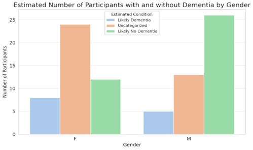
Dementia prediction by gender.
The kernel density estimates curves, or smooth lines, provide the histogram with a continuous, smoothed form. The general pattern in the age distribution for each ailment may be seen with the aid of these graphs.
This shows that both conditions (Likely Dementia and Likely No Dementia) are present over a broad age range, while there are some age bins where one condition may be more common than the other. A larger concentration of individuals in that age range who most likely do not have dementia is shown by the peak ages similar to the pink curve (Likely No Dementia), which appears to peak around the mid-60s. Although the blue curve (likely dementia) to be more dispersed, there are distinct peaks that point to the age groups when dementia is more common. Furthermore, there exist age ranges in which both estimated conditions overlap, suggesting that there exist persons within those age groups who, according to their MMSE scores, fall into both conditions. Based on the accuracy and MMSE scores results, here's the distribution of participants estimated to have “Likely Dementia” across different age groups:
40-49 years: 0 participants
50-59 years: 3 participants
60-69 years: 7 participants
70-79 years: 3 participants
80-89 years: 0 participants
From the data, the age group 60-69 years has the highest number of participants (7 participants) likely to have dementia based on their MMSE scores.
4.4. Comparison with Other Modalities
EEG and image modalities are compared in Tables 3 and 4, respectively, utilizing the suggested technique. The suggested approach for the EEG modality comparison uses Principal Component Analysis (PCA) for feature reduction in conjunction with a band-pass filter/noise filter (BPF/NF) and then clustering as a measure. This combination produced impressive results: 91% for Support Vector Machine (SVM) and 95% for Decision Tree (DT) and Random Forest (RF). The suggested approach shows a notable improvement in performance when contrasted with the other experiments in the table. This suggests that the feature extraction methods and filter selections in the suggested methodology are more successful for processing and analyzing EEG signals.
The great accuracy of the suggested approach is also attributed to its clustering metric. Though the use of clustering in the suggested methodology likely offers a more nuanced approach to understanding the underlying structure of the data, resulting in more accurate model training and prediction, traditional metrics like K-Fold cross-validation used in other studies are valuable for model validation.
Table 5 displays the speech modality; however, it does not list the characteristics or models that are utilized in the suggested approach, which makes it difficult to compare directly. However, if we assume that the novel method used in the EEG modality is also applied to speech, the success in EEG implies that such a tactic may also prove to be very successful in the voice modality. Even if they are outstanding, the accuracy revealed in the voice research using other approaches falls short of the high standard established by the suggested EEG methodology.
It is noteworthy that the effectiveness of the suggested methodology also suggests the significance of an integrated data analysis strategy in EEG signal processing. The suggested methodology establishes a new benchmark in the area by carefully choosing the filtering technique to preserve important signal components and lower noise, applying PCA for feature reduction to capture the most important signal features, and utilizing advanced machine learning models.
In summary, the suggested approach significantly outperforms conventional techniques in the EEG modality and probably will in the speech modality as well. Its merits are found in the thoughtful fusion of powerful statistical approaches with cutting-edge signal processing techniques, offering a path forward for future studies aiming at creating highly accurate classification systems in EEG signal processing.
CONCLUSION
Early-Onset Dementia
We acknowledge that our dataset primarily includes older adults, with participants ranging from 40 to 89 years old. Notably, the age group of 60-69 years has the highest number of participants, with seven individuals likely to have dementia based on their MMSE scores. This demographic focus may limit the generalizability of our findings to early-onset dementia. Future research should include a broader age range to address this limitation. Overall, the results point to the potential use of EEG signals as a non-invasive, reasonably priced substitute for established diagnostic techniques in the diagnosis and treatment of dementia. To confirm the results on a broader and more varied population and to examine the generalizability of the models across various dementia types and stages, additional study is necessary.
Real-World Applicability
The non-invasive nature of EEG makes this approach suitable for integration into portable EEG devices, enabling early diagnosis in clinical settings or even home environments. This could significantly improve patient care by facilitating timely interventions and treatment plans. Even yet, there are still certain restrictions. One key issue is that most approaches, for example, train traditional Machine Learning classifiers by extracting features from inputs that are merged within a single neural network. Another important drawback is that our research, in particular, trains EEG signals independently before using majority voting techniques, which considerably lengthens training time. Moreover, handling the tasks and events independently results in less-than-ideal performance. We also looked at the possibility that, even though EEG has yielded innovative outcomes in several domains, the process of detecting dementia with EEG data has not yet completely realized its potential.
Open Research Question
Dementia research is a vast and evolving field. While this study focuses on EEG-based diagnosis, other modalities like genetics, neuroimaging, and cognitive assessments hold promise for a comprehensive understanding of the disease. In summary, the suggested approach significantly outperforms conventional techniques in the EEG modality and probably will in the speech modality as well. Its merits are found in the thoughtful fusion of powerful statistical approaches with cutting-edge signal processing techniques, offering a path forward for future studies aiming at creating highly accurate classification systems in EEG signal processing.
Managerial Significance
Early and accurate diagnosis of dementia allows for better management of the disease and improved patient outcomes. This can translate to reduced healthcare costs by identifying patients who could benefit from early interventions and potentially delaying disease progression. Additionally, timely diagnosis empowers patients and caregivers to make informed decisions regarding treatment options, future planning, and potential support services. The focus of future research will be on the extraction and analysis of novel traits that are more likely to aid in dementia disease diagnosis. To improve accuracy, redundant and unnecessary features will also be eliminated from the present feature sets. The future study’s focus will also be on using digital filters or transforming analog signals to digital ones, which are currently missing in the present study. Future research will primarily focus on examining and contrasting the effectiveness of various trans-former designs, including GPT, T5, and XLNet, for dementia diagnosis and investigating the effectiveness of a multimodal transformer-based dementia diagnosis approach that combines text and voice data with additional modalities, like EEG and fMRI data.
DISCLOSURE
Part of this article has previously been published in the following work: Ahmed, Tanveer. (2023). “Detection of Dementia: Using Electroencephalography and Machine Learning.” [MASc Thesis], University of Victoria, CA. Available at: https://dspace.library.uvic.ca/server/api/core /bitstreams/1f6d1a0d-7c20-4cbd-b126-208df6c0bc8a/cont ent .
AUTHORS’ CONTRIBUTIONS
T.A., F.G., H.E., and M.E. contributed to conceptualization, T.A., F.G., H.E., and M.E. contributed to the performance and comparative analysis. T.A., F.G., H.E., and M.E contributed to resources and data curation.T.A wrote the draft. T.A., F.G., H.E., and M.E. helped in the investigation, and M.E. and F.G. helped in writing, reviewing, and editing. F.G., H.E., and M.E. supervised the study. All authors have read and agreed to the published version of the manuscript.
LIST OF ABBREVIATIONS
| AD | = Alzheimer Dementia |
| BPF | = Band Pass Filter |
| CV | = Cross Validation |
| DT | = Decision Tree |
| EEG | = Electroencephalography |
| HC | = Healthy Control |
| HPF | = High Pass Filter |
| LPF | = Low Pass Filter |
| LR | = Logistic Regression |
| ML | = Machine Learning |
| MMSE | = Mini-Mental State Examination |
| RF | = Random Forest |
| SVM | = Support Vector Machine |
AVAILABILITY OF DATA AND MATERIALS
All the data used in the manuscript were created and curated by us. Additionally, we used the Open Neuro Dataset for the EEG recordings [21].