Enhanced Multistructure Segmentation in 3D Whole-body MRI: A Comparative Evaluation of Deep Learning Architectures
Authors Info & Affiliations
Abstract
Introduction/Objective
Quantitative whole-body MRI relies on accurate delineation of multiple anatomical structures, yet manual labeling is slow and variable. We evaluate AISHANet, a deep learning model for multistructure 3D segmentation, and compare it with SegResNet, UNETR, and UNet using the same dataset split and evaluation protocol. The task covers 14 muscle groups and both lungs.
Methods
The dataset includes 100 whole-body DIXON T1 axial volumes acquired on a 3T Philips scanner (one volume per patient) with reference annotations produced by five expert radiologists. We used 80 volumes for training, 12 for validation, and 8 for testing. Performance was assessed with Dice Similarity Coefficient (DSC), directed Hausdorff distance, Sensitivity, ROC AUC, and F1-score. Metrics were computed per patient, macro-averaged across the 16 structures, and summarized as mean ± standard deviation (SD) across test patients.
Results
AISHANet obtained the highest overall scores, with a mean DSC 0.871 ± 0.017, directed Hausdorff distance in millimeters 24.11 ± 10.92, sensitivity 0.894 ± 0.047, ROC AUC 0.947 ± 0.024, and F1-score 0.871 ± 0.061. The best performance was observed in larger muscle groups (gluteus, thighs, calves), where DSC exceeded 0.88.
Discussion
While AISHANet consistently outperformed the baselines, performance decreased in anatomically challenging regions (abdomen and back), which are affected by lower contrast and thinner structures in axial views. Across models, we observed different failure modes: SegResNet tended to produce smoother masks, UNETR reduced isolated false positives, and UNet showed higher sensitivity to anatomical variability.
Conclusion
Under a controlled, single-protocol comparison, AISHANet provided the highest overall accuracy for multistructure whole-body MRI segmentation in this dataset. Remaining errors in low-contrast and anatomically complex regions motivate future work on improving robustness and validating performance across additional imaging settings, including other MRI scanner manufacturers and additional MRI sequence types.
1. INTRODUCTION
Whole-body MRI enables clinicians to perform quantitative assessment of body composition and musculoskeletal status for diagnosis and treatment planning. However, manual delineation of multiple muscle groups and lungs is time-consuming and subject to inter-reader variability. The integration of 3D segmentation can reduce inter-reader variability and speed up mask generation for volume- and morphology-based analyses, especially when structural changes in organs and muscles are associated with systemic conditions such as cirrhosis [1], cancer [2], heart dysfunction [3], and neurodegenerative diseases [4]. Automated muscle and fat segmentation techniques have demonstrated efficacy in providing reliable quantitative assessments of muscle volume and intramuscular fat content, which are relevant for the diagnosis and management of muscular dystrophies and other neuromuscular disorders [5]. Beyond the creation of patient-specific anatomical models for surgical planning, segmentation provides a basis for longitudinal quantification, allowing repeated measurements to be compared across time points to monitor disease course and treatment effects. Beyond its role in generating patient-specific models for precise surgical preparation, segmentation enables reliable longitudinal tracking to assess disease progression and treatment efficacy [6].
The value of muscle and organ segmentation in whole-body MRI has been demonstrated in numerous reported applications spanning diverse medical specialties. Commercial platforms, such as AMRA (Advanced MR Analytics), have already demonstrated how AI-based quantification of fat and muscle distribution can transform the management of metabolic and neuromuscular diseases [7, 8]. Because whole-body MRI datasets with multi-structure annotations remain scarce, evidence for segmentation architectures comes primarily from CT and PET/CT studies; nevertheless, these architectures are modality-agnostic and can be benchmarked under a unified protocol in MRI. SegResNet has been applied to 3D PET/CT segmentation tasks, and large-scale CT tools such as TotalSegmentator demonstrate that multi-structure delineation is feasible at the clinical scale. These CT and PET-CT studies motivate the choice of SegResNet and related backbones as strong baselines; however, their comparative performance on whole-body MRI-particularly for muscle groups and lungs-has been less systematically characterized [9-11].
MRI segmentation improves consistency and reduces manual effort for radiologists. Therefore, we perform a controlled comparison of UNet, SegResNet, and UNETR against our AISHANet on a whole-body DIXON T1 MRI dataset with 16 annotated structures (14 muscle groups and both lungs), using a single training and evaluation protocol. AISHANet combines residual-convolutional and self-attention encoders within a unified architecture to evaluate whether complementary representations improve segmentation performance. We assess whether AISHANet provides consistent gains over established baselines and discuss remaining limitations observed across anatomically challenging regions.
2. MATERIALS AND METHODS
2.1. Database
The study was conducted using a private, whole-body MRI dataset acquired on a 3T Philips system with a DIXON T1 axial protocol. To comply with the data owner’s proprietary requirements, specific acquisition parameters and vendor-specific implementation details are withheld. The data were provided in a fully anonymized format, so no direct identifiers were accessible to the authors. The cohort comprises adult participants (aged 20–60 years) with a balanced sex distribution, with consent and experimental protocols managed entirely by the data provider.
The study used 100 usable whole-body MRI volumes provided by the data owner. The final cohort resulted from an acquisition-site process of iterative protocol refinement and quality assurance, in which earlier scans that did not achieve the image quality required for consistent 3D annotation were screened out before data delivery.
Whole-body coverage was obtained by acquiring multiple stations per patient with region-specific receiver coils (head, abdomen, and lower limbs) following the scanner’s standard workflow. Data was received as station stacks and reconstructed into a single whole-body volume via rigid stack-wise concatenation (stitching) without non-rigid registration. Reference segmentations of the 16 target structures, which can be observed in Fig. (1), were created in 3D Slicer by five radiologists experienced in whole-body MRI interpretation. Prior to training, we performed an additional consistency check of the labels to confirm uniform class ordering and mapping throughout the dataset.
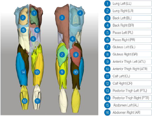
3D rendering of the reference annotations used for training. Expert radiologists delineated 16 structures (lungs; back; psoas; gluteus; anterior/posterior thighs; calves; abdomen), with distinct labels for left and right compartments. The figure shows the subject from both the front and the back to give an overview of the annotated regions.
2.2. Segmentation Networks
Image segmentation is a central component of many medical imaging pipelines, where accurate pixel/voxel assignment enables subsequent quantitative analysis. Given the range of anatomical appearances encountered in whole-body MRI, we compare representative convolutional and transformer-based architectures under a consistent experimental setting. Specifically, this section outlines UNet, SegResNet, UNETR, and AISHANet, with attention to the network features that matter for volumetric medical segmentation.
2.2.1. Unet
UNet is an encoder–decoder convolutional architecture with skip connections between corresponding resolution levels [12]. For volumetric segmentation, we used a 3D variant in which 2D operations are replaced by their 3D counterparts to process whole-volume inputs [13]. The contracting path applies repeated convolutional blocks with downsampling to learn multi-scale representations, whereas the expanding path performs upsampling and concatenates encoder features via skip connections to recover spatial detail. A final layer, 1 × 1 × 1 convolution, produces voxel-wise class predictions.
We include this model as a widely used convolutional baseline for biomedical segmentation. UNet-style architectures are widely used in MRI segmentation, including cardiac multi-structure segmentation evaluated on ACDC-style cine MRI datasets [14] and brain tumor segmentation studies using the BraTS benchmark [15].
2.2.2. Segresnet
SegResNet is a residual encoder–decoder architecture for volumetric semantic segmentation [16]. It follows a multi-resolution design in which the encoder learns hierarchical features using ResNet-like residual blocks, while the decoder progressively restores spatial resolution via upsampling to produce voxel-wise predictions. Residual connections facilitate optimization of deeper convolutional networks by improving feature propagation and gradient flow during training.
SegResNet has been evaluated as a baseline in multi-class tumor segmentation studies for radiotherapy-planning workflows [17]. It has also been used for lesion segmentation in whole-body PET/CT, including lymphoma detection and quantification benchmarks that directly compare SegResNet against other established architectures under a consistent evaluation protocol [18]. Finally, SegResNet has been included in benchmarking studies for fully automatic aortic root segmentation [19].
2.2.3. Unet Transformer (Unetr)
UNETR is a transformer-based architecture for 3D medical image segmentation that replaces the conventional CNN encoder with a Vision Transformer (ViT) operating on non-overlapping 3D patches. The input volume is partitioned into fixed-size patches, linearly embedded, and processed by stacked self-attention blocks to capture global context. Feature representations from intermediate transformer layers are reshaped and fused into a CNN decoder through skip connections, enabling progressive recovery of spatial detail and voxel-wise prediction via a final segmentation head [20].
UNETR was originally validated on public volumetric benchmarks, including BTCV multi-organ segmentation and selected Medical Segmentation Decathlon tasks, supporting its use as a transformer-based baseline for 3D segmentation under standardized protocols. Beyond the original benchmarks, UNETR has been used in practical volumetric multi-organ segmentation pipelines such as multi-organ segmentation for mouse embryo imaging, where UNETR serves as the underlying 3D segmentation model within a complete annotation and review workflow [21]. In parallel, transformer-based segmentation models have also been studied in multi-center settings where parameter-efficient adaptation strategies (e.g., prompt-based tuning) aim to preserve performance across institutions with limited re-training [22].
2.2.4. AISHANET
AISHANet is a hybrid 3D segmentation network that processes a volumetric input through two parallel encoders, followed by feature fusion and a SegResNet-style decoder. Let x ∈ RB×C×D×H×W denote the input tensor, where B is the batch size, C is the number of input channels, and D, H, and W are the depth (number of slices), height, and width of the 3D volume, respectively.
The residual–convolutional encoder builds a multiscale feature hierarchy using an initial 3D convolution and four encoder levels with residual blocks blocks_down = (1,2,2,4). The number of channels at level i is defined as Ci = init_filters · 2i Spatial downsampling is performed by stride-2 convolutions at levels i > 0, so that the encoder produces skip features at resolutions D × H × W, D/2 × H/2 × W/2, D/4 × H/4 × W/4, and a convolutional bottleneck at approximately D/8 × H/8 × W/8. If ndown= |blocks _down| denotes the number of encoder levels, then the convolutional bottleneck width is Cbot = init_filters · 2(ndown-1). The bottleneck representation is further refined by a feature-extraction projector consisting of normalization, a pointwise nonlinearity, and a 1 × 1 × 1 convolution, which preserves spatial resolution and channel width while improving feature conditioning prior to fusion.
In parallel, the self-attention encoder is a 3D Vision Transformer. The volume is partitioned into non-overlapping cubic patches of size p × p × p voxels; thus, D, H, and W are required to be divisible by p. Each patch is embedded into a latent representation of dimension , and the resulting token sequence is processed by a stack of transformer layers with num_heads attention heads and an MLP dimension mlp_dim. The transformer output tokens are reshaped back into a spatial feature grid of size (D/p) × (H/p) × (W/p). A second feature-extraction projector, implemented as a residual 3D convolutional block with kernel size (3 × 3 × 3), maps the transformer features from channels to the convolutional bottleneck width Cbot. The resulting attention feature volume is then aligned to the convolutional bottleneck spatial resolution via trilinear interpolation to match approximately (D/8) × (H/8) × (W/8).
The two aligned bottleneck tensors are integrated by a fusion module consisting of channel concatenation followed by a 1 × 1 × 1 convolution that reduces 2Cbot → Cbot, yielding a unified fused representation. Decoding follows a SegResNet-style upsampling path with blocks_up = (1,1,1): at each level, features are first projected with a 1 × 1 × 1 convolution (halving the number of channels), upsampled using a non-trainable interpolation mode, and then combined with the corresponding convolutional skip feature by element-wise addition, followed by residual refinement blocks. Finally, a normalization–activation– 1 × 1 × 1 convolution produces voxel-wise logits for K = out_channels segmentation classes. Figure 2 presents the block diagram of AISHANet, highlighting the feature-level ensemble of Residual-Convolutional and Self-Attention encoders and the shared decoder used to generate the final segmentation output.
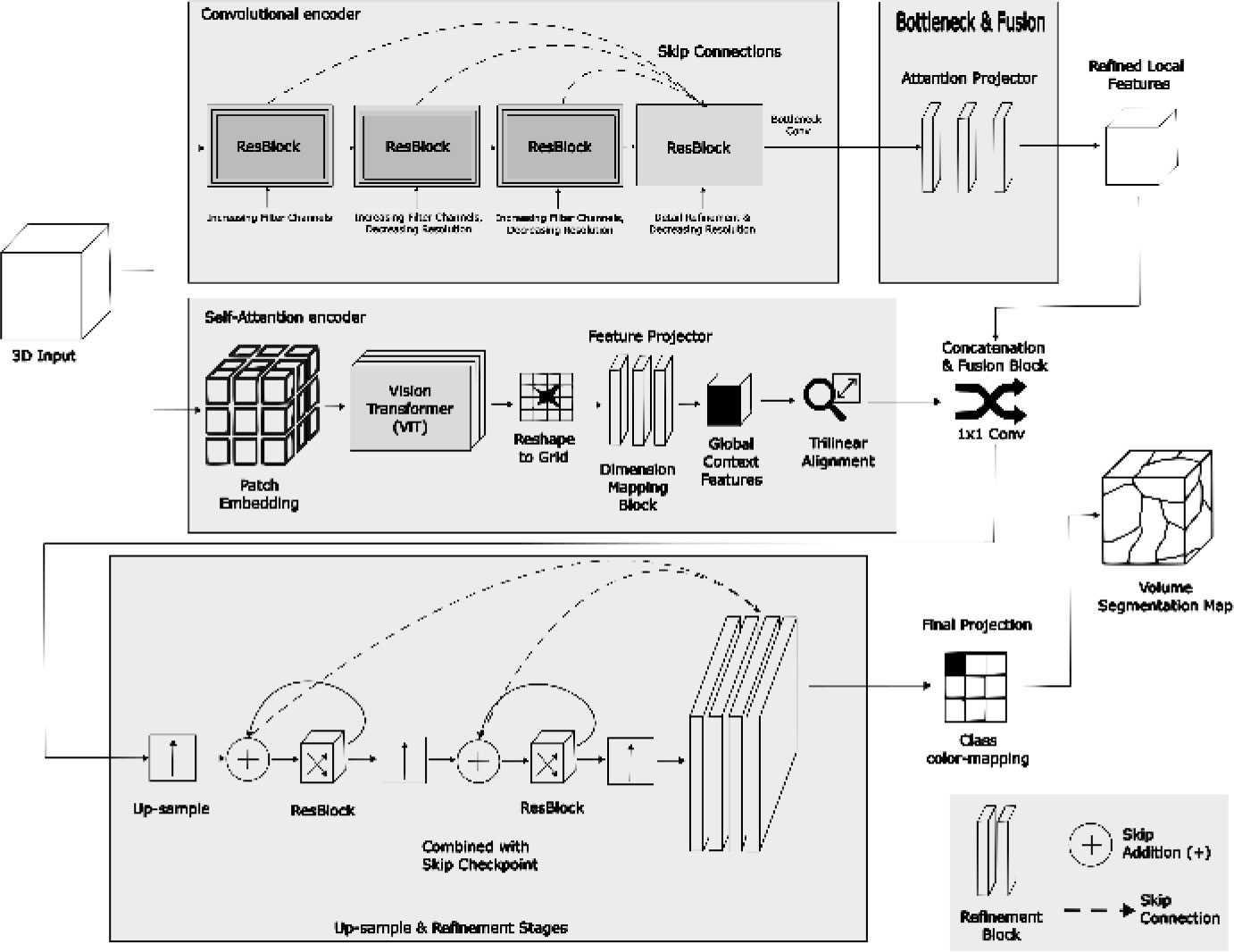
Block diagram of AISHANet, illustrating the feature-level ensemble of Residual-Convolutional and Self-Attention encoders. The fused features are processed through a shared decoder to produce the final segmentation output, leveraging the strengths of both encoders.
2.3. Statistical Analysis
All statistical analyses were performed in R. Segmentation performance was quantified using the Dice Similarity Coefficient (DSC) [23], directed Hausdorff distance [24], Sensitivity/Recall [25], ROC AUC [26], and F1-score [27]. Metrics were computed per patient and per target structure (14 muscle groups and both lungs). Overlap-based metrics (DSC, Sensitivity, and F1-score) were computed on hard labels obtained from voxel-wise class assignments. ROC AUC was computed in a one-vs-rest manner using flattened voxel-wise binary masks (ground truth vs predicted mask) derived from those hard labels.
For multi-class evaluation, ROC AUC and F1-score were computed in a one-vs-rest manner for each structure. Specifically, for each target structure , the voxel-wise score corresponded to the predicted probability for class , and reference labels were binarized as versus all remaining classes. Structure-wise results were then macro-averaged across the 16 structures to avoid dominance of larger structures in the overall summary. Summary statistics are reported as mean ± SD across patients.
DSC measures the overlap between the predicted segmentation and the ground truth segmentation, adding a small numerical stabilizer ∈. It was computed as:
where A represents the predicted segmentation, B represents the ground truth segmentation, and with ϵ = 1 × 10⁻⁴ used for numerical stability.
Directed Hausdorff distance complements overlap-based metrics by quantifying worst-case spatial disagreement between the predicted and ground-truth foreground voxels. Let A and B denote the sets of foreground voxel coordinates for the ground-truth and predicted masks, respectively, for a given structure. We computed the directed Hausdorff distance from A to B as:

where a and b are points (3D coordinates) in the sets A and B, respectively, and ||·||2 denotes the Euclidean norm, i.e., the largest Euclidean distance from any ground-truth voxel to its nearest predicted voxel. This directed formulation is sensitive to localized outlier mismatches and provides a complementary view of boundary/shape disagreement that may not be fully captured by overlap measures such as DSC. In our implementation, voxel indices were mapped to physical coordinates using the image voxel spacing from volume metadata; therefore, directed Hausdorff distances are reported in millimeters (mm) rather than voxel units.
Sensitivity (recall) assesses the fraction of true positive cases that the segmentation model successfully identified. It was computed as: The formula for sensitivity is:
where TP is the number of true positives and is the number of false negatives.
ROC AUC was computed independently for each anatomical structure in a one-vs-rest setting. For a given structure , the ground-truth mask was binarized voxel-wise as y = 1 for voxels belonging to k and y = 0 otherwise. The corresponding prediction was converted into a binary decision score map s Ɛ {0,1}, where s = 1 indicates voxels assigned to structure k by the final segmentation and s = 0 otherwise. The ROC curve was obtained by sweeping the decision threshold over the finite set of score levels (including an initial operating point representing an always-negative classifier), and computing the true positive rate (TPR) as TPR = TP / (TP + FN), also known as sensitivity or recall, versus the false positive rate (FPR) as FPR = FP / (FP + TN) at each threshold. The AUC was then calculated as the area under the resulting ROC curve using trapezoidal integration along the FPR axis. Because the decision scores are binary, the ROC curve contains a limited number of operating points and the resulting AUC is mathematically equivalent to the average of sensitivity (TPR) and specificity (TNR) for that structure, i.e., AUC = TPR + TNR/2.
The F1-score is the harmonic mean of precision and sensitivity (recall). It was calculated as:
where precision is defined as: Precision = TP / (TP + FP). These analyses allow a comparative evaluation of the segmentation accuracy, reliability, and clinical applicability of AISHANet, UNETR, SegResNet, and UNet.
To quantify uncertainty in the reported test-set metrics, we computed 95% confidence intervals using the bias-corrected and accelerated (BCa) bootstrap with 10,000 resamples [28]. Confidence intervals were obtained at the patient level, where each metric was first averaged across the 16 target structures for a given subject, and then summarized across subjects. BCa intervals were chosen because they provide improved finite-sample coverage by correcting for both bias and skewness in the bootstrap sampling distribution. Instead, we adopted an exact paired permutation (sign-flip) test on within-subject performance differences [29], enumerating all (2n) sign configurations to obtain exact values under minimal assumptions. We therefore emphasize effect sizes together with BCa confidence intervals as the main inferential summary and report exact permutation values as complementary evidence.
3. EXPERIMENTAL
A total of 100 annotated whole-body MRI volumes were available for model development. Data were split once at the patient level into training (n=80), validation (n=12), and test (n=8) sets. Because annotations were produced by multiple radiologists with unequal case contributions, the split was constructed to avoid concentrating labels from a single rater within a single subset; instead, each subset included cases annotated by all raters to reduce potential rater-source bias. The test set was held out and used only for final evaluation.
Whole-body volumes were reconstructed from multiple station acquisitions (stacks) with partial overlap. Stacks were concatenated using rigid stack-wise stitching guided by spatial metadata to prevent duplicated anatomy in the overlap region. Prior to model training, all volumes were verified to be readable and correctly oriented within the training pipeline.
Reference annotations for the 16 target structures (14 muscle groups and both lungs) were produced in 3D Slicer by five radiologists experienced in whole-body MRI interpretation. Segmentations were performed slice-by-slice with optional use of 3D Slicer interpolation tools to accelerate delineation, followed by multi-planar review (axial/sagittal/coronal) and 3D inspection when needed. An internal annotation guide specified the target structures, label definitions, and anatomical boundaries. Additional quality control was performed by the research team to verify anatomical plausibility and label integrity (e.g., correct class mapping and ordering). Minor label issues were corrected programmatically, while structural delineation issues were returned for rater correction; overall, only a small fraction of cases required such interventions.
All models were trained and evaluated under an identical protocol to enable a controlled, architecture-agnostic comparison. Training was performed using patch-based learning on cubic sub-volumes sampled from the full whole-body scans. Before sampling, volumes were cropped to the foreground region, and patches of size 96 × 96 × 96 were then extracted using a balanced positive/negative strategy (pos:neg = 1:1, 5 samples per volume, batch size = 2). On-the-fly augmentation was applied throughout training and included geometric perturbations (random flips along two axes with p = 0.25, random 90° rotations with p = 0.1 and up to k = 3, continuous rotations up to approximately 0.3 - 0.4 rad per axis with p = 0.75, and random zoom with p = 0.75 in the range 0.7 - 1.7), as well as appearance transformations (contrast adjustment with y = 0.2 - 2.5 and p = 0.4 , Gaussian noise with σ = 0.03 and p = 0.2, intensity shifts with offset = 0.30 and p = 0.25, histogram shifts with 10–20 control points and p = 0.3, plus occasional smoothing/sharpening). To further regularize learning, we also used coarse local shuffling (25 holes, spatial size = 16, p = 0.25). These augmentation settings were selected to emulate plausible variability encountered in real-world whole-body MRI acquisitions, including differences in patient positioning, minor motion, field-of-view and scaling changes, and intensity/contrast fluctuations and noise across scanners and protocols. Optimization used Adam with an initial learning rate of 1 × 10⁻³, a 30-epoch warm-up, and a cosine decay schedule bounded by 1 × 10⁻⁵, with scheduled restarts of the optimizer during training. During training, validation Dice was computed on discretized predictions (argmax followed by one-hot encoding) and included the background class for monitoring purposes. The training objective combined Dice and cross-entropy terms using an unweighted formulation (equal trade-off between Dice loss and cross-entropy, with no additional class re-weighting) by minimizing a composite criterion defined as (1 - mean Dice) + L_train, where mean Dice is the aggregated validation Dice and L_train is the epoch-averaged training loss. Models were trained for 600 epochs with validation every 10 epochs; both the final checkpoint (“last”) and the best checkpoint (“best”) were saved, where “best” was selected using a composite criterion combining validation mean Dice and training loss. For inference, full-volume predictions were obtained with a sliding-window strategy using the same 96 × 96 × 96 ROI and a sliding-window batch size of .
4. RESULTS
Overall test-set performance is summarized in Table 1, and qualitative examples are shown in Fig. (3). AISHANet achieved the highest macro-averaged DSC (0.871 ± 0.017), Sensitivity (0.894 ± 0.047), ROC AUC (0.947 ± 0.024), and F1-score (0.871 ± 0.061) and the lowest directed Hausdorff distance in milimeters (24.11 ± 10.92). In terms of boundary errors, this corresponds to a reduction in worst-case spatial deviation relative to all baselines, which showed substantially larger directed Hausdorff distances (UNet 54.64 ± 52.93, UNETR 53.48 ± 53.02, and SegResNet 34.17 ± 16.10). Relative to the strongest baseline in each metric, AISHANet improved DSC by compared with UNETR (0.813 ± 0.031) and increased Sensitivity by +0.129 compared with SegResNet (0.765 ± 0.168). Similarly, ROC AUC increased by +0.065 over SegResNet (0.882 ± 0.084), and F1-score improved by +0.111 over SegResNet (0.760 ± 0.128).
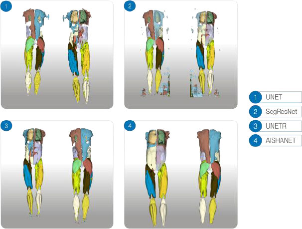
Qualitative 3D comparison for a single test-set subject. Results are shown in a 2×2 grid: UNet and SegResNet (top row), UNETR and AISHANet (bottom row). Each panel includes anterior and posterior views; opacity was adjusted in selected structures to improve internal visualization.
Across baselines, UNETR showed higher DSC than UNet and SegResNet (Table 1), but did not improve Sensitivity compared with UNet (both 0.170 on average). This suggests that, under one-vs-rest scoring and argmax-based hard labels, UNETR’s higher overlap did not translate into higher recall, consistent with more conservative predictions that match the target region when detected but may still miss portions of the structure.
| Model | DSC | Hausdorff | Sensitivity | ROC AUC | F1-score |
|---|---|---|---|---|---|
| UNet | 0.726 ± 0.029 | 54.64 ± 52.93 | 0.710 ± 0.222 | 0.855 ± 0.111 | 0.756 ± 0.183 |
| SegResNet | 0.760 ± 0.032 | 34.17 ± 16.10 | 0.765 ± 0.168 | 0.882 ± 0.084 | 0.760 ± 0.128 |
| UNETR | 0.813 ± 0.031 | 53.48 ± 53.02 | 0.710 ± 0.195 | 0.868 ± 0.097 | 0.758 ± 0.155 |
| AISHANet | 0.871 ± 0.017 | 24.11 ± 10.92 | 0.894 ± 0.047 | 0.947 ± 0.024 | 0.871 ± 0.061 |
Structure-wise results for AISHANet are reported in Table 2. Performance was strongest for the lungs and for large muscle groups, including gluteus, thighs, and calves (DSC ≈ 0.89 - 0.92), with consistently high ROC AUC values (0.94 - 0.97). In contrast, abdomen and back muscles yielded the lowest DSC values (e.g., abdomen left/right 0.76 - 0.78 and back left/right 0.80 - 0.81) and the largest variability (SD ≈ 0.05 - 0.06), matching the visually challenging regions shown in Fig. (4). While Table 2 presents the exact numerical values of the structure-wise evaluation, Fig. (4) provides a complementary visual summary that highlights relative performance differences and variability across anatomical structures. Such visualization facilitates the identification of patterns across structures and supports a more intuitive interpretation of the results discussed in the following sections. Directed Hausdorff distances provide additional insight into these region-dependent errors. Despite lower overlap in Abdomen/Back, the directed Hausdorff distances remained in a moderate range (Abdomen Left 21.15 ± 7.53 mm, Abdomen Right 27.74 ± 11.69 mm, Back Left 34.82 ± 6.61 mm, Back Right 33.41 ± 5.78 mm), suggesting that predictions typically remain within the correct compartment but are limited by boundary delineation. In contrast, the thigh compartments illustrate a complementary behavior: posterior thigh achieved high overlap (DSC ≈ 0.91–0.92) while showing comparatively larger directed Hausdorff distances (Posterior Thigh Left 38.00 ± 2.89 mm, Posterior Thigh Right 34.70 ± 5.50 mm), consistent with occasional outlier deviations that are not fully reflected by overlap metrics.
| Class | DSC | Hausdorff | Sensitivity | ROC AUC | F1-score |
|---|---|---|---|---|---|
| Lung Left (LL) | 0.90 ± 0.00 | 20.21 ± 19.67 | 0.91 ± 0.05 | 0.96 ± 0.03 | 0.90 ± 0.00 |
| Lung Right (LR) | 0.91 ± 0.01 | 23.09 ± 15.50 | 0.90 ± 0.06 | 0.95 ± 0.03 | 0.91 ± 0.01 |
| Back Left (BL) | 0.81 ± 0.05 | 34.82 ± 6.61 | 0.87 ± 0.03 | 0.93 ± 0.01 | 0.81 ± 0.05 |
| Back Right (BR) | 0.80 ± 0.06 | 33.41 ± 5.78 | 0.86 ± 0.02 | 0.93 ± 0.01 | 0.80 ± 0.06 |
| Psoas Left (PL) | 0.83 ± 0.03 | 15.53 ± 6.11 | 0.85 ± 0.06 | 0.92 ± 0.03 | 0.84 ± 0.02 |
| Psoas Right (PR) | 0.85 ± 0.02 | 14.87 ± 5.22 | 0.87 ± 0.06 | 0.93 ± 0.03 | 0.85 ± 0.02 |
| Gluteus Left (GL) | 0.92 ± 0.01 | 14.18 ± 1.26 | 0.93 ± 0.02 | 0.96 ± 0.01 | 0.92 ± 0.01 |
| Gluteus Right (GR) | 0.91 ± 0.01 | 17.35 ± 8.44 | 0.92 ± 0.01 | 0.96 ± 0.01 | 0.91 ± 0.02 |
| Anterior Thigh Left (ATL) | 0.89 ± 0.02 | 22.83 ± 9.09 | 0.92 ± 0.02 | 0.96 ± 0.01 | 0.89 ± 0.02 |
| Anterior Thigh Right (ATR) | 0.89 ± 0.02 | 24.82 ± 9.86 | 0.92 ± 0.03 | 0.96 ± 0.01 | 0.89 ± 0.02 |
| Calf Left (CL) | 0.91 ± 0.02 | 21.22 ± 9.01 | 0.93 ± 0.03 | 0.96 ± 0.01 | 0.91 ± 0.01 |
| Calf Right (CR) | 0.92 ± 0.02 | 21.82 ± 4.48 | 0.94 ± 0.02 | 0.97 ± 0.01 | 0.92 ± 0.02 |
| Abdomen Left (AL) | 0.76 ± 0.05 | 21.15 ± 7.53 | 0.88 ± 0.01 | 0.94 ± 0.01 | 0.77 ± 0.05 |
| Abdomen Right (AR) | 0.78 ± 0.04 | 27.74 ± 11.69 | 0.84 ± 0.03 | 0.92 ± 0.01 | 0.78 ± 0.04 |
| Posterior Thigh Left (PTL) | 0.91 ± 0.02 | 38.00 ± 2.89 | 0.90 ± 0.02 | 0.95 ± 0.01 | 0.91 ± 0.02 |
| Posterior Thigh Right (PTR) | 0.92 ± 0.01 | 34.70 ± 5.50 | 0.89 ± 0.02 | 0.94 ± 0.01 | 0.92 ± 0.01 |
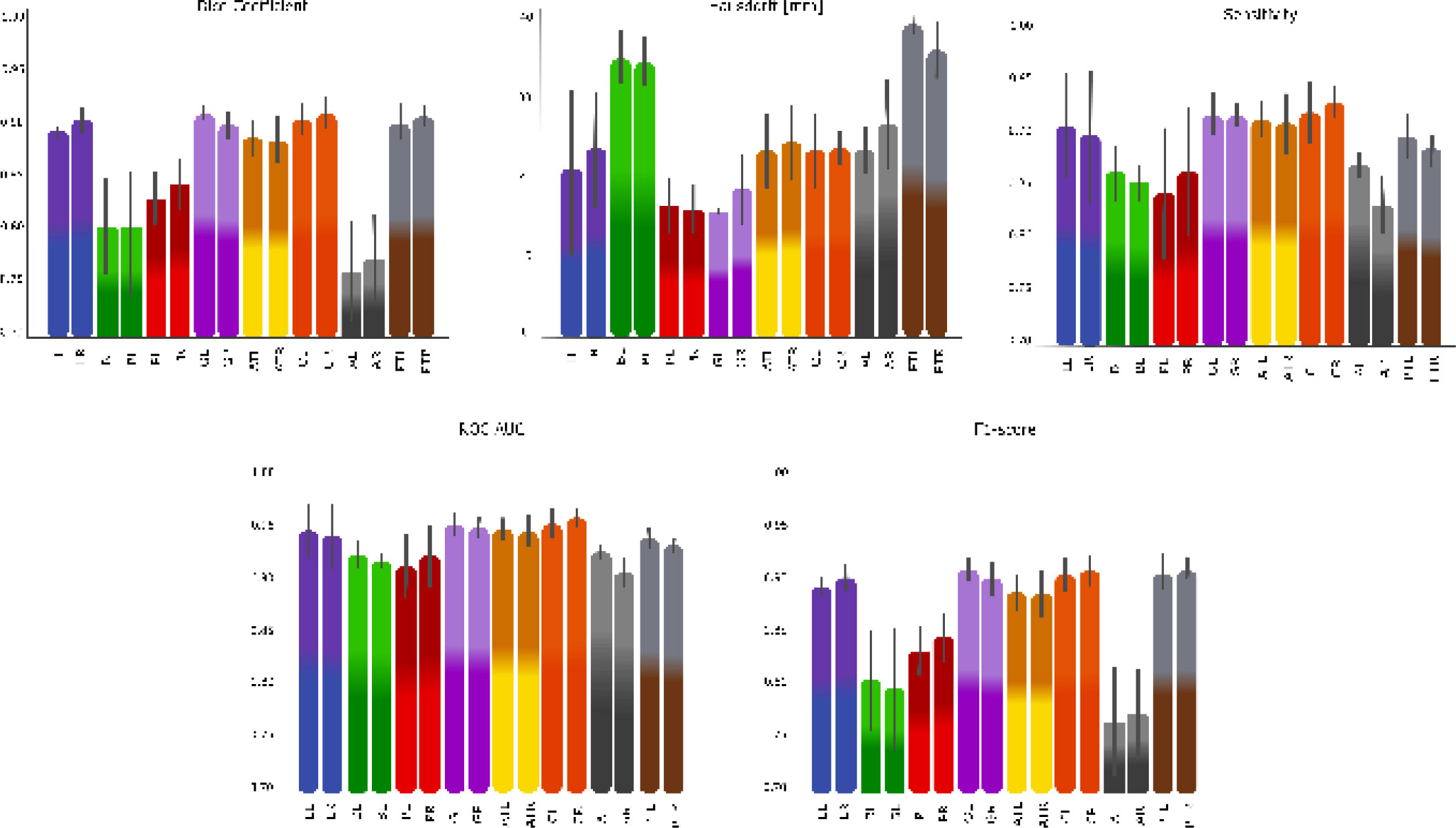
Segmentation performance metrics (DSC, directed Hausdorff distance, Sensitivity, ROC AUC, and F1-score) for AISHANet across the anatomical structures: Lung Left (LL) and Lung Right (LR), Back Left (BL) and Back Right (BR), Psoas Left (PL) and Psoas Right (PR), Gluteus Left (GL) and Gluteus Right (GR), Anterior Thigh Left (ATL) and Anterior Thigh Right (ATR), Calf Left (CL) and Calf Right (CR), Abdomen Left (AL) and Abdomen Right (AR), Posterior Thigh Left (PTL) and Posterior Thigh Right (PTR).
Global test-set performance with uncertainty estimates is reported in Table 3. AISHANet achieved the strongest overall results across all metrics, with DSC 0.87 [0.85, 0.89], Sensitivity 0.89 [0.88, 0.91], ROC AUC 0.95 [0.94, 0.95], and F1-score 0.87 [0.85, 0.89]. In terms of boundary errors, AISHANet also produced the lowest directed Hausdorff distance, 24.11 mm [14.51, 28.83], indicating reduced worst-case spatial deviation compared with the baselines. Among the baseline models, UNETR showed the highest overlap (DSC 0.81 [0.79, 0.84]), while SegResNet achieved higher recall than UNETR (Sensitivity 0.84 [0.81, 0.88]) but with lower overlap (DSC 0.76 [0.73, 0.79]). Overall, the uncertainty intervals support a consistent advantage for AISHANet in both overlap-based performance and boundary consistency.
| Model |
DSC (mean [CI95]) |
Hausdorff (mean [CI95]) |
Sensitivity (mean [CI95]) |
ROC AUC (mean [CI95]) |
F1-score (mean [CI95]) |
|---|---|---|---|---|---|
| UNet | 0.7 [0.71, 0.75] |
40.72 [35.27, 52.08] |
0.71 [0.70, 0.73] |
0.86 [0.85, 0.87] |
0.76 [0.74, 0.78] |
| SegResNet | 0.76 [0.73, 0.79] |
38.85 [27.62, 55.48] |
0.84 [0.81, 0.88] |
0.92 [0.91, 0.94] |
0.84 [0.82, 0.86] |
| UNETR | 0.81 [0.79, 0.84] |
53.48 [38.32, 64.24] |
0.71 [0.65, 0.77] |
0.87 [0.84, 0.89] |
0.76 [0.74, 0.79] |
| AISHANet | 0.87 [0.85, 0.89] |
24.11 [14.51, 28.83] |
0.89 [0.88, 0.91] |
0.95 [0.94, 0.95] |
0.87 [0.85, 0.89] |
5. DISCUSSION
Performance differences across structures were not uniform. While large muscle groups and lungs achieved consistently high overlap (e.g., gluteus and calves with DSC around 0.91–0.92), lower DSC values were observed for the Abdomen and Back classes (DSC ≈ 0.76–0.78 and 0.80–0.81, respectively; Table 2). Importantly, these lower overlaps occurred despite relatively high Sensitivity and ROC AUC in the same regions, suggesting that the model often detects the target class but struggles to place accurate boundaries in anatomically constrained areas. This interpretation is further supported by the directed Hausdorff results: Abdomen/Back shows reduced overlap while maintaining moderate worst-case distances, which is consistent with boundary imprecision rather than gross mislocalization. Conversely, thigh structures maintain high overlap but can still exhibit elevated directed Hausdorff distances, indicating that occasional localized outliers (e.g., small regions of anterior–posterior confusion) may persist even when the overall compartment is well captured.
A plausible explanation is the combination of limited conspicuity and partial-volume effects in thin muscles on axial whole-body MRI. When muscle layers are only a few voxels thick, small boundary shifts translate into a noticeable DSC drop, and a single voxel may contain mixed tissue signal, reducing separability from adjacent fat [30]. These challenges are well recognized in lumbar/paraspinal MRI segmentation, where both manual delineation and automated approaches report difficulty in defining borders in the presence of narrow structures and variable appearance [31, 32]. Whole-body acquisitions also bring practical sources of region-dependent variability (residual motion, as well as subtle discontinuities at station boundaries) that are not uniformly expressed across the body. In DIXON-based protocols, these effects can be amplified in the abdomen due to respiratory motion and local field-related intensity variations, whereas they tend to be less prominent in the thigh or calf regions. This helps contextualize why errors concentrate in the abdomen/back, while performance remains more stable for larger, higher-contrast muscle groups. While our discussion centers on MRI, CT body-composition studies similarly note that abdominal fat distribution can mask muscle interfaces, reinforcing that the abdomen is a difficult compartment across modalities [33].
A simple structure-wise stratification reinforces this pattern across metrics. Here, “structure-wise” refers to the 16 target classes evaluated individually, grouped qualitatively by anatomical size and boundary visibility. High and stable performance was observed in well-defined compartments such as the lungs, gluteus, and calves, where overlap (DSC/F1) is high, and both sensitivity and one-vs-rest ROC AUC remain consistently strong, with moderate directed Hausdorff distances. Intermediate behavior was observed for the psoas and anterior thigh groups, where overlap remains relatively high, but small boundary shifts can affect DSC. The most challenging structures were the abdomen and back muscles, which show the lowest overlap yet retain relatively high sensitivity/ROC AUC, consistent with compartment detection but imperfect boundary delineation in thin, low-contrast regions.
In addition to the structure-level patterns, uncertainty estimates help interpret how stable these differences are at the cohort level. The confidence intervals in Table 3 add context to the average scores by showing that performance differences are not only reflected in DSC and F1-score, but also in boundary behavior. The directed Hausdorff distance exhibits wider uncertainty than overlap metrics, especially for UNet and UNETR, which is expected for worst-case distance measures that are sensitive to localized outliers. In this setting, AISHANet combines higher overlap with a markedly lower directed Hausdorff distance, suggesting that its gains are not limited to improved detection but extend to more consistent spatial placement of the segmentation. The baseline patterns are also informative: SegResNet attains comparatively high sensitivity but lags behind in DSC, which is compatible with segmentations that capture more positives yet remain less well-aligned with the ground truth; UNETR, in contrast, improves overlap but does not increase sensitivity and shows higher Hausdorff distances, consistent with conservative predictions that may miss portions of structures and produce occasional spatial deviations. Finally, because the evaluation set is limited, we intentionally prioritize uncertainty intervals and effect sizes over rank-based significance testing; the reported CIs provide a transparent view of variability and help avoid over-interpreting p-values that would be unstable under very small paired samples.
Overall, the results indicate that AISHANet provides strong average performance, but boundary accuracy in thin, low-contrast regions remains the main failure mode. Future work will focus on strategies that explicitly target boundary definition in these compartments (e.g., region-aware sampling during training, boundary-focused objectives, or light post-processing to remove discontinuities), while preserving the consistent performance observed in well-defined structures.
CONCLUSION
In this study, we performed a controlled comparison of UNet, SegResNet, and UNETR against our proposed AISHANet on a private whole-body DIXON T1 MRI dataset with 16 annotated structures (14 muscle groups and both lungs), using the same train/validation/test partition and the same evaluation protocol across models. Under these conditions, AISHANet achieved the best overall performance across overlap-, discrimination-, and boundary-based criteria, with the highest macro-averaged DSC, Sensitivity, ROC AUC, and F1-score, and the lowest directed Hausdorff distance. These results support the practical value of hybrid designs that combine convolutional feature extraction with self-attention to integrate local boundary cues and broader anatomical context when segmenting multiple targets in whole-body MRI, while also motivating future work to confirm robustness on larger and more diverse cohorts and acquisition settings.
Beyond the overall averages, the structure-wise results provide a clearer interpretation of the model’s behavior. AISHANet was consistently strong in larger, well-defined compartments-lungs, gluteus, thighs, and calves-while the remaining errors were largely concentrated in anatomically constrained regions such as the abdomen and back muscles. This suggests that the main limitation is not that the model fails to find the correct compartment, but that it sometimes places boundaries imperfectly when structures are thin or have low contrast. Directed Hausdorff patterns are consistent with this view, suggesting predominantly boundary-level errors in Abdomen/Back, while highlighting that occasional localized outlier deviations can still occur in thigh compartments despite high overlap. This is also in line with the relatively high one-vs-rest ROC AUC values across structures, even when overlap-based metrics decrease in Abdomen/Back. In practical terms, this helps prioritize what to improve next: focusing on boundary refinement in the abdomen/back is more likely to move the needle than changes aimed at gross detection, while preserving the stable performance already achieved in larger compartments.
The baseline comparison, observed in Fig. (5), also showed that different architectures fail in different ways under the same protocol. In Fig. (5), the directed Hausdorff distance was min–max normalized for visualization (the largest observed value was mapped to 1.0, and the remaining values were scaled proportionally), since all other metrics are naturally bounded in . In our setting, SegResNet tended to produce smoother masks and, in some cases, higher recall. UNETR, by contrast, often produced cleaner outputs with fewer isolated false positives, but under argmax-based hard labels, this did not consistently convert into higher sensitivity or better overlap. These complementary behaviors offer a reasonable explanation for the hybrid strategy behind AISHANet and support the broader idea that combining local texture-sensitive cues with global context can reduce failure modes that matter in whole-body segmentation.
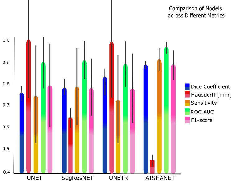
Comparative performance of AISHANet, UNETR, SegResNet, and UNet across the proposed evaluation metrics. Bars show the mean ± SD across the analyzed anatomical structures. For visualization, the directed Hausdorff distance was normalized by scaling all values relative to the maximum observed distance (max = 1.0), enabling direct comparison with metrics bounded in .
From a clinical perspective, reliable segmentation of muscle groups and lungs can support downstream quantitative analyses in several scenarios. Repeated measurements of psoas, gluteal, and thigh muscles can enable body-composition monitoring and objective tracking of changes during treatment or rehabilitation. Likewise, consistent abdominal-region muscle delineation can contribute to quantitative follow-up in spine-related workflows. Importantly, these are potential uses of automated segmentation and should be validated prospectively in the intended clinical context.
Two practical constraints should be considered when interpreting these findings. First, the held-out evaluation set comprised 8 patients, reflecting the cost and logistical burden of acquiring and manually annotating whole-body MRI at scale. Second, all volumes were acquired using the same scanner and DIXON T1 protocol; therefore, external validation is required to quantify robustness to domain shift across scanners, protocols, and sites. In addition, whole-body coverage required multi-station acquisitions that were reconstructed by rigid stack-wise concatenation (stitching) without non-rigid registration, which can introduce subtle intensity discontinuities and boundary artifacts at station transitions. More broadly, vendor- and site-dependent reconstruction and post-processing differences (e.g., coil combination, intensity scaling, and Dixon reconstruction variants) may alter contrast distributions and affect generalization beyond the present setting. As a partial mitigation, we designed the training protocol to include intensity- and contrast-oriented augmentation to emulate plausible inter-stack and acquisition variability; however, confirming robustness across vendors and institutions remains an important next step. Finally, no formal inter-rater agreement study was performed because each case was annotated once under the constraints of the data-collection budget; nevertheless, annotations followed an internal guide and underwent multi-planar review and consistency checks to ensure label integrity.
From a deployment standpoint, AISHANet is computationally feasible for volumetric inference: in our configuration, whole-body inference completed in approximately 50 seconds, with GPU memory usage driven primarily by the sliding-window size (up to ~6 GB VRAM in our setup). These characteristics are compatible with practical post-acquisition processing, while leaving room for optimization depending on the target hardware and throughput requirements.
Consistent with the above constraints, no external dataset was available under the current proprietary data-sharing agreement; therefore, the present study is intended as a controlled single-site baseline. Future work will focus on (i) establishing collaborations that enable multi-vendor and multi-institution validation and (ii) evaluating harmonization or post-processing strategies tailored to cross-scanner variability. In parallel, methodological improvements should prioritize boundary definition in thin, low-contrast structures-particularly in Abdomen/Back-while also reducing rare outlier regions in thigh compartments, for example, by improving the separation between anterior and posterior thigh groups through region-aware sampling, boundary- or surface-oriented objectives, and/or light post-processing that enforces anatomical plausibility. Complementary evaluation beyond overlap metrics (e.g., boundary distances or volumetric agreement), together with stratified analyses by body-composition factors, may further clarify the clinical relevance of segmentation differences in narrow compartments.
Overall, the findings indicate that AISHANet provides consistent gains over established convolutional and transformer-based baselines for multi-structure segmentation in 3D whole-body MRI under a unified evaluation protocol, while also clarifying that abdomen and back musculature remain the dominant failure mode to address for broader clinical deployment.
AUTHORS’ CONTRIBUTIONS
The authors confirm their contribution to the paper as follows: R.D-P.: Conceptualization; Formal analysis; Supervision; Writing – original draft; G.G.: Methodology; Resources; Validation; Investigation; Data curation; Writing – original draft; F.T.R.: Conceptualization; Formal analysis; Software; Investigation; Visualization; Data curation; Writing – original draft; B.E.R.: Conceptualization; Resources; Project administration; Writing – review & editing; J.O.: Conceptualization; Project administration; Writing – original draft; J.P.R-G.: Conceptualization; Validation; Funding acquisition; Project administration; J.A.G-C.: Formal analysis; Software; Writing – review & editing; C.A.R.H.: Investigation; Visualization; Software. All authors reviewed the results and approved the final version of the manuscript.
LIST OF ABBREVIATIONS
| 3D | = Three-dimensional |
| SD | = Standard Deviation |
| AI | = Artificial intelligence |
| MRI | = Magnetic resonance imaging |
| 3T | = Three Tesla |
| T1 Dixon | = T1-weighted Dixon MRI sequence |
| CNN | = Convolutional neural network |
| DSC | = Dice similarity coefficient |
| ROC | = Receiver operating characteristic |
| ROC AUC | = Area under the ROC curve |
| TP | = True positive |
| TN | = True negative |
| FP | = False positive |
| FN | = False negative |
| TPR | = True positive rate |
| FPR | = False positive rate |
| CT | = Computed tomography |
| PET | = Positron emission tomography |
| PET/CT | = Positron emission tomography–computed tomography |
| ALS | = Amyotrophic lateral sclerosis |
| UNAM | = Universidad Nacional Autónoma de México |
| PAPIIT | = Programa de Apoyo a Proyectos de Investigación e Innovación Tecnológica |
| AMRA | = Advanced MR Analytics |
| AISHANet | = Proposed hybrid 3D whole-body MRI segmentation model. |
ETHICS APPROVAL AND CONSENT TO PARTICIPATE
The original study protocol, including participant recruitment, MRI acquisition, and informed-consent procedures, was reviewed and approved by the Ethics Committee of Hospital Ángeles, Mexico City, Mexico.
HUMAN AND ANIMAL RIGHTS
All human-data procedures adhered to relevant institutional and national standards and to the Declaration of Helsinki.
AVAILABILITY OF DATA AND MATERIALS
The MRI dataset is privately held by the data provider and cannot be released publicly due to confidentiality and proprietary constraints. Model weights and implementation details are likewise not publicly distributed. Access requests, if any, must be addressed to the data owner and would be subject to their internal review and approval requirements.
FUNDING
This study was supported by Universidad Nacional Autónoma de México (UNAM), Mexico through PAPIIT grants IN108624 and IT101624. The funders had no involvement in study design, data acquisition, analysis, or interpretation, the publication decision, or manuscript writing.
CONFLICT OF INTEREST
Some authors are affiliated with AISHA, the developer of the proposed model; this is disclosed as per journal policy. No other competing interests are declared.
ACKNOWLEDGEMENTS
Declared none.
APPENDIX A
Appendix A reports the same per-structure breakdown for all baselines. Notably, the abdomen and back were also the lowest-performing structures for UNet, SegResNet, and UNETR (e.g., UNet abdomen right DSC 0.60 and back DSC ~ 0.67; SegResNet abdomen DSC ~0.67 - 0.68; UNETR abdomen DSC ~0.71 - 0.74), indicating that these regions drive a substantial portion of the residual error across architectures. Compared with the best baseline per structure, AISHANet produced the largest DSC gains on the posterior thigh right (+0.10) and lungs (+0.07 - 0.09), while improvements were smaller for already wellperforming structures such as gluteus and anterior thigh (≈ +0.02 -0.03). Detailed per-structure results for all models are provided in Tables A1 to A3 in Appendix A.
This appendix provides per-structure results for UNet, SegResNet, and UNETR. For each class, we report mean ± SD for DSC, Sensitivity, ROC AUC, and F1-score. These tables support the main comparison by highlighting structure-dependent differences and variability across cases.
| Class | DSC | Hausdorff | Sensitivity | ROC AUC | F1-score |
|---|---|---|---|---|---|
| Lung Left (LL) | 0.72 ± 0.01 | 81.40 ± 72.04 | 0.77 ± 0.24 | 0.83 ± 0.12 | 0.81 ± 0.17 |
| Lung Right (LR) | 0.72 ± 0.01 | 32.21 ± 13.53 | 0.73 ± 0.25 | 0.85 ± 0.13 | 0.79 ± 0.17 |
| Back Left (BL) | 0.67 ± 0.06 | 47.15 ± 6.63 | 0.73 ± 0.22 | 0.86 ± 0.11 | 0.70 ± 0.21 |
| Back Right (BR) | 0.67 ± 0.07 | 143.9 ± 124.7 | 0.72 ± 0.21 | 0.83 ± 0.11 | 0.69 ± 0.22 |
| Psoas Left (PL) | 0.73 ± 0.03 | 36.37 ± 42.20 | 0.62 ± 0.25 | 0.83 ± 0.13 | 0.75 ± 0.19 |
| Psoas Right (PR) | 0.73 ± 0.03 | 19.20 ± 8.20 | 0.64 ± 0.25 | 0.82 ± 0.13 | 0.75 ± 0.18 |
| Gluteus Left (GL) | 0.80 ± 0.01 | 21.94 ± 3.59 | 0.78 ± 0.21 | 0.89 ± 0.11 | 0.84 ± 0.17 |
| Gluteus Right (GR) | 0.74 ± 0.02 | 16.04 ± 3.60 | 0.77 ± 0.20 | 0.86 ± 0.10 | 0.84 ± 0.17 |
| Anterior Thigh Left (ATL) | 0.76 ± 0.02 | 48.17 ± 34.24 | 0.78 ± 0.22 | 0.90 ± 0.11 | 0.76 ± 0.17 |
| Anterior Thigh Right (ATR) | 0.79 ± 0.03 | 28.51 ± 7.02 | 0.77 ± 0.22 | 0.85 ± 0.11 | 0.79 ± 0.19 |
| Calf Left (CL) | 0.78 ± 0.02 | 30.48 ± 10.31 | 0.73 ± 0.23 | 0.87 ± 0.11 | 0.76 ± 0.17 |
| Calf Right (CR) | 0.76 ± 0.02 | 37.24 ± 12.46 | 0.72 ± 0.20 | 0.88 ± 0.10 | 0.79 ± 0.17 |
| Abdomen Left (AL) | 0.65 ± 0.06 | 73.57 ± 46.67 | 0.61 ± 0.21 | 0.84 ± 0.10 | 0.64 ± 0.21 |
| Abdomen Right (AR) | 0.60 ± 0.05 | 115.1 ± 56.9 | 0.62 ± 0.22 | 0.85 ± 0.11 | 0.67 ± 0.20 |
| Posterior Thigh Left (PTL) | 0.76 ± 0.02 | 54.07 ± 39.61 | 0.70 ± 0.22 | 0.84 ± 0.11 | 0.75 ± 0.17 |
| Posterior Thigh Right (PTR) | 0.73 ± 0.02 | 70.26 ± 45.16 | 0.69 ± 0.21 | 0.87 ± 0.10 | 0.76 ± 0.17 |
| Class | DSC | Hausdorff | Sensitivity | ROC AUC | F1-score |
|---|---|---|---|---|---|
| Lung Left (LL) | 0.81 ± 0.01 | 53.02 ± 30.53 | 0.77 ± 0.19 | 0.90 ± 0.10 | 0.77 ± 0.11 |
| Lung Right (LR) | 0.81 ± 0.02 | 35.46 ± 10.58 | 0.77 ± 0.20 | 0.91 ± 0.10 | 0.75 ± 0.12 |
| Back Left (BL) | 0.68 ± 0.05 | 47.22 ± 6.10 | 0.73 ± 0.16 | 0.85 ± 0.08 | 0.73 ± 0.16 |
| Back Right (BR) | 0.65 ± 0.07 | 45.42 ± 11.11 | 0.72 ± 0.16 | 0.87 ± 0.08 | 0.71 ± 0.16 |
| Psoas Left (PL) | 0.69 ± 0.04 | 24.25 ± 18.22 | 0.72 ± 0.20 | 0.83 ± 0.10 | 0.72 ± 0.13 |
| Psoas Right (PR) | 0.71 ± 0.04 | 19.69 ± 6.83 | 0.73 ± 0.21 | 0.89 ± 0.10 | 0.69 ± 0.13 |
| Gluteus Left (GL) | 0.81 ± 0.02 | 19.97 ± 7.25 | 0.78 ± 0.16 | 0.88 ± 0.08 | 0.80 ± 0.11 |
| Gluteus Right (GR) | 0.82 ± 0.02 | 13.80 ± 1.85 | 0.81 ± 0.14 | 0.85 ± 0.08 | 0.78 ± 0.12 |
| Anterior Thigh Left (ATL) | 0.78 ± 0.03 | 34.12 ± 9.48 | 0.78 ± 0.16 | 0.91 ± 0.08 | 0.82 ± 0.12 |
| Anterior Thigh Right (ATR) | 0.81 ± 0.03 | 25.86 ± 7.05 | 0.77 ± 0.17 | 0.92 ± 0.09 | 0.83 ± 0.12 |
| Calf Left (CL) | 0.83 ± 0.02 | 29.37 ± 13.59 | 0.81 ± 0.17 | 0.91 ± 0.08 | 0.80 ± 0.12 |
| Calf Right (CR) | 0.84 ± 0.02 | 31.03 ± 11.06 | 0.81 ± 0.15 | 0.91 ± 0.08 | 0.82 ± 0.12 |
| Abdomen Left (AL) | 0.68 ± 0.06 | 42.80 ± 14.02 | 0.76 ± 0.15 | 0.84 ± 0.07 | 0.67 ± 0.16 |
| Abdomen Right (AR) | 0.67 ± 0.05 | 38.56 ± 9.83 | 0.74 ± 0.17 | 0.85 ± 0.09 | 0.69 ± 0.15 |
| Posterior Thigh Left (PTL) | 0.80 ± 0.03 | 37.72 ± 14.07 | 0.79 ± 0.16 | 0.89 ± 0.08 | 0.78 ± 0.12 |
| Posterior Thigh Right (PTR) | 0.78 ± 0.02 | 48.35 ± 14.67 | 0.75 ± 0.15 | 0.90 ± 0.07 | 0.80 ± 0.11 |
| Class | DSC | Hausdorff | Sensitivity | ROC AUC | F1-score |
|---|---|---|---|---|---|
| Lung Left (LL) | 0.81 ± 0.02 | 73.24 ± 72.39 | 0.71 ± 0.21 | 0.84 ± 0.10 | 0.76 ± 0.15 |
| Lung Right (LR) | 0.84 ± 0.02 | 31.96 ± 18.08 | 0.74 ± 0.23 | 0.85 ± 0.12 | 0.79 ± 0.14 |
| Back Left (BL) | 0.75 ± 0.06 | 50.15 ± 17.11 | 0.68 ± 0.19 | 0.88 ± 0.09 | 0.68 ± 0.18 |
| Back Right (BR) | 0.74 ± 0.07 | 133.95 ± 127.03 | 0.66 ± 0.18 | 0.87 ± 0.09 | 0.69 ± 0.19 |
| Psoas Left (PL) | 0.78 ± 0.03 | 35.62 ± 33.25 | 0.68 ± 0.23 | 0.88 ± 0.11 | 0.73 ± 0.15 |
| Psoas Right (PR) | 0.79 ± 0.03 | 26.20 ± 9.58 | 0.63 ± 0.23 | 0.90 ± 0.11 | 0.73 ± 0.15 |
| Gluteus Left (GL) | 0.90 ± 0.01 | 26.94 ± 9.41 | 0.74 ± 0.18 | 0.91 ± 0.10 | 0.82 ± 0.14 |
| Gluteus Right (GR) | 0.89 ± 0.02 | 23.29 ± 14.42 | 0.71 ± 0.17 | 0.89 ± 0.09 | 0.79 ± 0.15 |
| Anterior Thigh Left (ATL) | 0.86 ± 0.02 | 54.67 ± 38.96 | 0.75 ± 0.19 | 0.90 ± 0.09 | 0.79 ± 0.15 |
| Anterior Thigh Right (ATR) | 0.87 ± 0.03 | 37.76 ± 7.04 | 0.76 ± 0.20 | 0.87 ± 0.10 | 0.78 ± 0.15 |
| Calf Left (CL) | 0.86 ± 0.02 | 21.73 ± 14.20 | 0.79 ± 0.20 | 0.84 ± 0.10 | 0.79 ± 0.15 |
| Calf Right (CR) | 0.83 ± 0.02 | 40.24 ± 17.97 | 0.80 ± 0.18 | 0.86 ± 0.09 | 0.81 ± 0.15 |
| Abdomen Left (AL) | 0.74 ± 0.05 | 78.32 ± 50.97 | 0.71 ± 0.18 | 0.87 ± 0.09 | 0.65 ± 0.18 |
| Abdomen Right (AR) | 0.71 ± 0.05 | 126.1 ± 56.86 | 0.64 ± 0.20 | 0.85 ± 0.10 | 0.69 ± 0.17 |
| Posterior Thigh Left (PTL) | 0.83 ± 0.03 | 43.82 ± 47.95 | 0.70 ± 0.19 | 0.86 ± 0.10 | 0.80 ± 0.15 |
| Posterior Thigh Right (PTR) | 0.82 ± 0.02 | 70.26 ± 39.16 | 0.66 ± 0.18 | 0.84 ± 0.09 | 0.82 ± 0.14 |