Mathematical Model of the Process of Ultrasonic wave Propagation in a Relax Environment with its Given Profiles at three Time Moments
Abstract
Objective:
The process of ultrasound oscillations in a relaxed environment, provided that the profiles of the acoustic wave at three time moments are known, is modeled by a three-point problem for the partial differential equation of the third order in time. This equation as a partial case contains a hyperbolic equation of the third order, which is widely used in ultrasound diagnostics.
Methods:
The differential-symbol method is applied to study a three-point in-time problem. The advantage of this method is the possibility to obtain a solution of the problem only through operations of differentiation.
Results:
We propose the formula to construct the analytic solution of the problem, which describes the process of ultrasound oscillations propagation in a relax environment. Due to this, the profile of the ultrasonic wave is known at any time and at an arbitrary point of space. The class of quasi-polynomials is distinguished as a class of uniqueness solvability of a three-point problem.
Conclusion:
Using the proposed method, it is possible to analyze the influence of the main parameters of ultrasound diagnostics problems on the propagation of acoustic oscillations in a relaxed environment. The research example of a specific three-point problem is given.
1. INTRODUCTION
To describe the processes of various natures, there are many models which are considered basic parameters of the process and they can effectively be investigated by mathematical methods.
Moreover, the same type of models is often used in completely different fields of knowledge. For example, in modeling biomechanical and medical processes [1-3], developed models for problems of hydromechanics and gas dynamics are used [4, 5]. One of the important areas of mathematical modeling is the simulation of processes by differential equations, which is used, in particular, in modeling the processes of wave propagation. Thus it is possible to predict their behavior depending on propagation conditions. In particular, the property of ultrasonic waves to change the speed of their propagation and absorption with any changes in the environment is taken into account. This property, as well as the reflection of the ultrasonic wave at the boundaries of different environments in the human body, are the basis of the ultrasound diagnostics, which is one of the most informative methods of non-invasive diagnosis in medicine. It is widely used to diagnose the work of organs and obtain their three-dimensional images, accelerate metabolic processes in the body and destroy various tumors.
Today, more and more mathematical models of mechanical, biomedical and geophysical processes are used not only in partial differential equations of the second order in time, but also the third and fourth orders in time [6-9]. For studying these models, there are applied numerical, qualitative and asymptotic methods [10, 11].
The Cauchy problem for hyperbolic equation of a third-order in time of the form
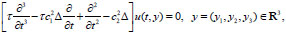 |
(1) |
is investigated [12-14]. The problems of ultrasonic diagnostics contain the Eq. (1) in which u(t, y) is dynamic pressure, Δ is three-dimensional Laplace operator, constants c1 and c2 are limiting phase velocities of sound, τ is relaxation time.
In addition to the Cauchy problem for partial differential equations with initial conditions, problems with other time conditions are also intensively investigated. In particular, there are multipoint problems in which values of the unknown solution are given at different times. Problems with multipoint time conditions in unbounded domains are studied [15, 16], and in bounded domains with additional conditions of spatial variables are also studied [17-20].
Multipoint in time problems has an important physical interpretation and these are problems in which the states of the process are given at
2. METHODS
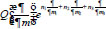
In the present paper, the differential-symbol method is applied. This method has been successfully used to solve the problems for partial differential equations with time-variable conditions in unbounded domains. Such problems are the Cauchy problem as well as the problem with local and nonlocal multipoint in time conditions. To solve these problems, the Fourier transform method, which allows us to find solutions in integral form, in particular, in the form of improper integrals of given functions, is traditionally used. In contrast to the Fourier transform, the differential-symbol method makes it possible to construct solutions of the previous problems using differentiation operations. If the right-hand sides of conditions (for example, the initial functions in the Cauchy problem) are quasipolynomials φi (x) then the solutions of the problem are represented in a form of actions of differential expressions
 on certain functions of a parameter or a vector-parameter ν. After the actions of these differential expressions, the parameter ν is assumed to be zero.
3. RESULTS
3.1. Posing of the Problem
Eq. (1) of ultrasound oscillations by replacement x =(c1τ)−1y, α= (с2)−1c1 is transformed into the one-parameter (parameter
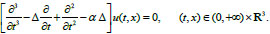 |
(2) |
The mathematical model of the process of ultrasound wave propagation which contains Eq. (2) and the profile of oscillation is given at three equidistant moments of time t = jh, where
 0 (Eq. 3):
 |
(3) |
is considered [13]. In the presented paper, we obtain more general results.
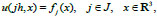
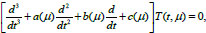
Let us consider the problem for the partial differential equation of the third order (Eq. 4).
 |
(4) |
Which describes not only ultrasound waves as Eq. (2), but also different waves depending on the operator coefficients
 and
and
 , where
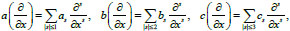 |
(5) |
 are complex numbers (Eq. 5).
The profiles of wave are given at time moments t0, t1, t2 by conditions (Eq. 6):
 |
(6) |
Let us find a solution to problem (4)-(6) using the differential-symbol method [22].
According to Eq. (4), the ordinary differential equation with parameter μ has the form (Eq. 7):
 |
(7) |
where
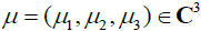 .
.
To simplify the form of formulas, we will write a = a (μ), b = b (μ), c=c(μ). Let us denote the roots of the characteristic (cubic) equation (Eq. 8):
 |
(8) |
by
 . These roots have the following image (Eq. 9):
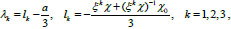 |
(9) |
Where
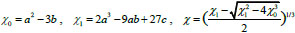 and the cubic root of the one
 belongs to the second quarter.
If the determinant

Of the polynomial
 does not equal zero, then Eq. (8) has simple roots, moreover, if
for a2 ≠ 3b and λ1 = λ2 = λ3 = −a/3 for a2 3b.
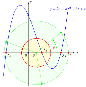
For real numbers a, b, c if D ≥ 0 there are real roots (if D > 0 they are different) and if D < 0 we get real and two complex roots.
The geometric interpretation of the real roots is given in Fig. (1), where
 |
is the set of roots and σ = S+ i Imσ ϵ C, φϵ [0,2π/3), r≥0 (we have a double root
 for φ = 0, φ = π / 3 and a triple root S for r = 0).
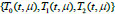
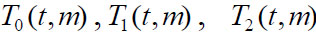
For the equation of the third order (7) with the coefficients, which is integered by the vector-parameter μ, we write the normal fundamental at the point t 0 system of the solutions
 which is defined uniquely. In addition, we find the fundamental system
 of solutions of Eq. (7), which satisfy conditions
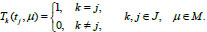 |
(10) |
The system
 can be constructed only for vectors
 for which the following condition
 |
(11) |
is realized.
Therefore,
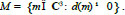 |
(12) |
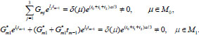
Set M, which is defined by formula (12), is divided in three sets
 , moreover for vectors μ ϵ M0 roots of Eq (8) are simple, for μ ϵ M1 there are simple and double roots among the roots of Eq. (8) and a triple root for vectors μ ϵ M2.
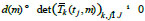
Let us consider the array
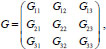 , which has the form
and array
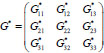 of the form
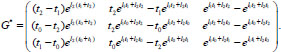
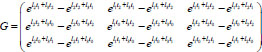
If μ ϵ M 0 (simple roots), then
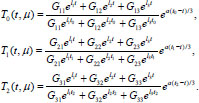 |
(13) |
For the case μ ϵ M1 (root λ1 is simple and λ2 is double), then
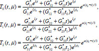 |
(14) |
Eqs (13, 14) are correct (determinants are nonzero) because m = 1,2,3 and we have
For the case μ ϵ M2 (triple root) formulas of the elements of the fundamental system of solutions of Eq. (7), which satisfy conditions (10) are simplified and take the form
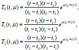 |
(15) |
We introduce the quasipolynomial functions of the form
 |
(16) |
where Q(x) is nonzero polynomial of variables x1, x2, x3 with complex coefficients, ν1, ν2, ν3 are complex numbers, moreover, the vector ν = (ν1, ν2, ν3) satisfies the condition δ(ν) = 0, i.e. ν ϵ M where M is the set (12).
For the set (12), KM is a class of functions which consists of the quasipolynomials of variables x1, x2, x3 which can be represented as a finite sum of quasipolynomials of the form (15) with the different vectors. Also, we suppose that the zero quasipolynomial g(x) = 0 belongs to KM.
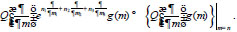
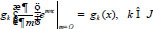
For each quasipolynomial of the form (15), the differential expression
 can be obtained by replacing the vector x with the vector-derivative
 . The differential expression
 of the infinite order acts on the analytic function γ(μ) at the neighborhood of m= n by the formula
Similarly, we determine the effect of differential expressions of infinite order on the analytic functions for more general quasipolynomials of the class KM. We also assume that
 ≡ 0 for g = 0.
3.2. Main result
For arbitrary functions g 0(x), g1(x), g2(x) from the class KM there is a unique solution of the problem (4), (6), which is represented by the formula
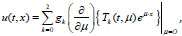 |
(17) |
moreover, u(t,.) ϵ KM for all t ϵ (0,∞).
In Eq. (17) we assume O = (0,0,0)
 .
.
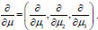
The fact that function (17) satisfies the partial differential Eq. (4) follows from the commutativity of the differentiation operators
 ,
,
 , and that the functions
 satisfy the ordinary differential Eq. (7).
For the function of the form (17) three-point conditions (6) are carried out, since
satisfy conditions (10) and the equalities
 |
are realized.
The solution of three-point problem (4), (6) in the class of quasipolynomials for each fixed t ϵ (0,∞) belongs to KM, is unique. This is proved by differential-symbol method (see, for example [23],). Choice of the functions g 0(x), g1 (x), g2 (x) from class KM is significant.
Obviously, if the functions g 0 (x), g1 (x), g2 (x) in conditions (6) belong to the set KM, then according to Eq. (17), the solutions of problem (4), (6) are quasipolynomials.
Numerous studies [26-30] have been devoted to the construction of solutions of some partial differential equations and boundary value problems for these equations in the form of quasipolynomials.
Thus, the process of oscillation propagation, in particular, ultrasound wave in a relaxed environment with given wave profiles at three points at time is investigated.
The process is modeled by the problem (4), (6) for the partial differential Eq. (4) of the third order in time with three-point time conditions (6). The method of constructing the solution of problem (4), (6) is indicated. The class of quasipolynomials
3.3. Example of Research of the Process of Ultrasound wave Propagation with its given Profiles at three Moments of Time
Let us investigate the process of acoustic oscillations using the proposed method for a specific example.
Example. We study the process of propagation of an ultrasound wave in relax environment, which is described by problem (4), (6) with the following parameters:
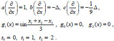 |
The profile of wave at the moment of time t=1 is a sum of two quasipolynomials of the form (16) that is
 |
in which the polynomials are
 respectively, then the vector-parameters in the exponent are equal to
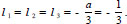
 and −ν. These vectors ν and −ν belong to the set M2 and the corresponding root of Eq. (8) is triple:
 |
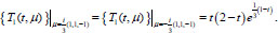
Function (14) take the form
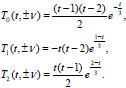 |
Since
 , then

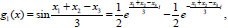
The solution of problem (4), (6) with given parameters can be found by Eq. (16):
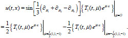 |
We calculate
 |
Finally, we obtain the solution to the problem
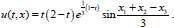 |
Let us investigate the solution of the problem on parallel planes x1 + x2-x3 - 3h = 0 of the space R3, where
 . Then the solution of problem has the form (Eq. 18):
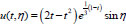 |
(18) |
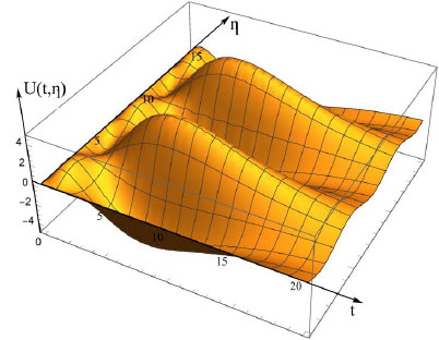
and it is 2p-periodic function by variables h.
The graph of the function (18) of two variables t and h is given in Fig. (2).
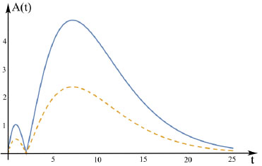
Therefore, function (17) describes the periodic oscillations of the ultrasound wave with the period T = 2π by the variable η. For
 the amplitudes of oscillation are given in the following form:
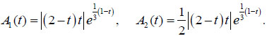 |
These amplitudes are shown in Fig. (3) by a solid and dashed line.
As mentioned above, the found solution of problem is unique in the class of quasipolynomials and belongs to KM each fixed t. Therefore, the ultrasound wave oscillates in a limited range at any time and exponentially goes to zero for
 on planes which is parallel to the plane x1 + x2-x3 = 0 and acquire zero values on the planes
 .
.
4. DISCUSSION
It should be noted that in recent years the approaches in which differentiation operations are used instead of integration operations, which are more complex (see, for example, [31, 32]). In these works, instead of the integration operation, other formulas which provide for the operation of differentiation by parameter
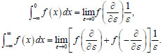 |
To calculate the Laplace transform
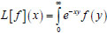 of the function f(x) there is proposed the following formula
 |
in which a differentiation by the variable x is used.
Therefore, the method which is proposed in this article is a new and effective method of solving the problem with three-point in time conditions.
CONCLUSION
The process of ultrasound wave propagation in the environment with relaxation under the condition of setting the wave profile at three points of time is simulated by the three-point problem for a partial differential equation of the third order in time.
A class of functions in which there is a unique solution to the problem has been established. It is a class of quasipolynomials with certain conditions on the index in exponents. An effective method for constructing a solution to the problem in this class is proposed. The process of acoustic oscillations is studied for a specific example. In the future, it is interesting to study acoustic oscillations under the influence of external forces, which leads to the study of the problem with three point in time conditions for a nonhomogeneous partial differential equation of the third order in time.
The proposed research results can be used in biomechanics and medicine, in particular, in the theory of ultrasound diagnostics.
ETHICS APPROVAL AND CONSENT TO PARTICIPATE
Not applicable.
HUMAN AND ANIMAL RIGHTS
No humans and animals were used for studies that are the basis of this research.
CONSENT FOR PUBLICATION
Not applicable.
AVAILABILITY OF DATA AND MATERIALS
Not applicable.
FUNDING
None.
CONFLICT OF INTEREST
The authors declare no conflict of interest, financial or otherwise.
ACKNOWLEDGEMENTS
Declared none.