A New Deep Learning Model based on Neuroimaging for Predicting Alzheimer's Disease
Authors Info & Affiliations
Abstract
Background:
The psychological aspects of the brain in Alzheimer's disease (AD) are significantly affected. These alterations in brain anatomy take place due to a variety of reasons, including the shrinking of grey and white matter in the brain. Magnetic resonance imaging (MRI) scans can be used to measure it, and these scans offer a chance for early identification of AD utilizing classification methods, like convolutional neural network (CNN). The majority of AD-related tests are now constrained by the test measures. It is, thus, crucial to find an affordable method for image categorization using minimal information. Because of developments in machine learning and medical imaging, the field of computerized health care has evolved rapidly. Recent developments in deep learning, in particular, herald a new era of clinical decision-making that is heavily reliant on multimedia systems.
Methods:
In the proposed work, we have investigated various CNN-based transfer-learning strategies for predicting AD using MRI scans of the brain's structural organization. According to an analysis of the data, the suggested model makes use of a number of sites related to Alzheimer's disease. In order to interpret structural brain pictures in both 2D and 3D, the Alzheimer's Disease Neuroimaging Initiative (ADNI) dataset includes straightforward CNN designs based on 2D and 3D convolutions.
Results:
According to these results, deep neural networks may be able to automatically learn which imaging biomarkers are indicative of Alzheimer's disease and exploit them for precise early disease detection. The proposed techniques have been found to achieve an accuracy of 93.24%.
Conclusion:
This research aimed to classify Alzheimer's disease (AD) using transfer learning. We have used strict pre-processing steps on raw MRI data from the ADNI dataset and used the AlexNet, i.e., Alzheimer's disease has been categorized using pre-processed data and the CNN classifier.
1. INTRODUCTION
Like many significant populations around the world, India's massive population, which is the second largest in the world, is faced with the problem of aging. Alzheimer's disease is a dreadful degenerative condition that can strike anyone at any time and continue to do so until it exacts its ultimate, fatal toll. In India, more than 4 million people suffer from dementia [1]. The disease, which affects at least 6 million people globally, is a global health emergency that requires attention. Alzheimer's disease is the main factor contributing to dementia. Amnesia is one of the symptoms of AD, a chronic brain disease that has a detrimental effect on a patient's quality of life. Other symptoms include difficulties in thinking, problem-solving, or speaking. A chronic neurological condition known as AD usually begins gradually and progresses over time. Moreover, the cause of AD is not well known. While some treatments could momentarily lessen symptoms, none can stop or reverse the disease's course. The majority of AD cases are still found in advanced stages when treatment will only stall the progression of cognitive impairment [2].
Enhancing preventative and disease-modifying drugs requires early AD detection. Some persons may develop moderate cognitive impairment (MCI) during the onset of Alzheimer's disease, a period that occurs between the normal loss of ageing psychological traits and the additional severe deterioration of dementia. It suggests a modest cognitive and memory deficiency, but it has little bearing on how well the person performs on a daily basis and is infrequently observed in clinical settings. Recent research has revealed that MCI patients are more likely than normal individuals to develop the AD epidemic [3]. The support vector machine is most frequently employed to diagnose AD. To allow clinical design automation, SVM builds prognosticative classification models using high-dimensional, instructional imaging alternatives. However, the majority of feature extraction ideas entail arduous manual extraction from a semi-automatic brain structure sketch that takes a long time and is computationally challenging to perform.
In a variety of fields, such as speech recognition, computer vision, spoken language understanding, and more recently, medical analysis, deep learning algorithms, a distinct family of machine learning approaches, deliver the greatest results (Lecun et al., 2015). Because they can automatically determine the optimal method to represent data from raw images without the need for feature selection beforehand, deep learning algorithms differ from typical machine learning techniques in that they make the process more unbiased and less subject to prejudice [4-6]. Therefore, deep learning algorithms are better at spotting both minor and significant anatomical defects. Recently, deep learning was successfully used on the Alzheimer's Disease Neuroimaging Initiative (ADNI) dataset to distinguish between AD patients and healthy controls. It has only been demonstrated to predict AD development within 1.5 years in MCI patients using ADNI auxiliary MRI controls and deep learning calculations without the prior assessment of elements (considering dim issue [GM] volumes as a contribution). For the diagnosis of multi-modal neuroimaging knowledge supported by AD/MCI, recent advances in MRI, PET, and other machine-learning approaches have been made [7-10]. Over the past ten years, photo categorization issues have been rather successfully addressed using convolutional neural networks. Despite the fact that a number of extremely effective CNN image classifiers, such as AlexNet and ResNet, are built to support vast amounts of training data, this is unsuitable for medical image classification due to a lack of resources, especially for brain tomography.
Following is the organization of the remaining portions of this paper; Section 2 presents the related work. The suggested work is defined in Section 3 of the document. The result analysis and discussion are presented in Section 4. Future works are included in Section 5.
2. RELATED WORK
MCI, which can progress into AD, is predicted by a model created by Jin Liu et al. and Wang [1]. They first selected a small number of regions using AAL (automated anatomical labelling), a program and digital atlas of the human brain with a labelled volume that maps the brain and labels its many regions. Wang presented an MCI model that might be converted into AD [2]. Functional magnetic resonance imaging (fMRI) data from the resting state was used by Ronghui Ju, Chenhui Hu, Pan-Zhou, and Quanzheng Li [3]. The resting-state functional magnetic resonance imaging (R-fMRI) data are processed into a 90-130 matrix that keeps the key information, with the brain being divided into 90 regions. The strength of the relationships is assessed using the Pearson correlation coefficient [4, 5].
A system based on a convolutional neural network (CNN) was created by Gang Guo, Min Xiao, Min Du, and Xiaobo Qu [6-9] to precisely predict the mild cognitive impairment (MCI) transformation into Alzheimer's disease (AD) using data from MRI. When MRI images are processed, age correction is the first thing used. Marcia Hon and Naimul Mefraz Khan [10] attempted to address a number of fundamental issues, including the requirement for a large number of training images and the necessity to improve CNN's structure adequately. Prospective MCI decliners can be distinguished utilising the method created by Babajani-Feremi et al. [11] for identifying AD using structural and functional MRI integration. The classic statistical analysis approach suggested by Fei Guo et al. [12] was built on the multi-scale time series kernel-based learning model, which was utilised to detect brain abnormalities. They discovered that this technique is useful for precisely identifying brain disorders. Xia-an Bi et al. [13] identified HC, patients' aberrant brain areas, and AD by building a random neural network cluster based on fMRI data. Modupe Odusami et al. [14] developed a model for early-stage identification of functional deficits in MRI images using ResNet18. Impedovo et al. [15] introduced a protocol. This technique provided a “cognitive model” for assessing the connection between cognitive processes and handwriting for both healthy participants and patients with cognitive impairment. A 3D CNN architecture was used by Harshit et al. [16, 17] to characterise the four stages of AD [AD, early MCI (EMCI), late MCI (LMCI), and normal control (NC)] using 4D FMRI images. Additionally, Dan et al. [18] and Silvia et al. [17] suggested additional CNN structures for 3D MRI-based categorization of distinct AD stages. Juan Ruiz et al. [19, 20] used the 3D densely linked convolutional network (3D DenseNet) to categorise items in 3D MRI scans in four different ways. According to a recent study by Nichols et al. [21], there are currently 57.4 million dementia sufferers globally, and by the year 2050, there may be as many as 152.8 million. Early diagnosis is crucial for treating patients effectively and halting the condition's progression [22]. In order to address the minor sample issue, uncover abnormality in the brain, and identify pathogenic genes in multimodal data from the AD Neuroimaging Initiative (ADNI), Bi et al. [23] proposed clustering evolutionary random forest design. LeNet-5 is a model that Yang and Liu [24] recommend adopting for classification and prediction. PET imaging was performed on 350 ADNI individuals with MCI. The model obtained sensitivity and specificity in MCI transformation prediction of 91.02 and 77.63%, respectively [17, 24].
A lot of infrastructure that can enable AD detection and medical picture categorization has recently been developed. However, the literature has not adequately addressed these subjects. Using other cutting-edge methods covered in the section of ‘Related Work’, it is possible to organise the uniqueness of this study as follows:
• The early diagnosis of Alzheimer's disease and the classification of medical images are performed using an end-to-end framework. The recommended method handles 2D and 3D structural brain MRI and is based on basic CNN architecture. The underpinning for these designs is convolution in 2D and 3D.
• Four AD stages have been investigated utilising three multi-class and twelve binary medical picture classification systems.
• Due to the COVID-19 outbreak, it was difficult for individuals to routinely visit hospitals in order to prevent gatherings and infections, while the experimental results demonstrated high performance according to performance indicators.
3. METHOD
3.1. Architecture
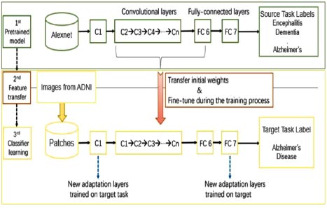
The basic architecture of the proposed work is shown in Fig. (1). The proposed work consisted of three models. Firstly, the pre-trained AlexNet model was trained on MRI scans of different diseases related to the brain, like dementia, tumor, encephalitis, Parkinson’s, Alzheimer’s, etc. This was done due to the lack of training datasets available to train our machine. In the second phase, the features of the existing pre-trained model were transferred to a new AlexNet model. In the third phase, images were taken from the ADNI dataset to train and fine-tune our model, which has been designed specifically for Alzheimer’s disease prediction. The process is described in detail in the latter part of the paper.
3.2. Data Acquisition
In this study, the convolutional neural network (CNN) classifier has been built using the MRI images from the Alzheimer's Disease Neuroimaging Initiative (ADNI) [1]. ADNI is actually an ongoing study that was started in 2004. It aims at comprehending the diagnostic and prognosticative terms of Alzheimer's disease-specific biomarkers. The information enclosed an overall 715 structured MRI scans out of both ADNI1 as well as ADNI2 phases, having 320 AD cases and 395 normal controls. Then, the data were acquired for the dataset with the previously mentioned description in the DICOM MRI format. For further investigation of the information, it was required to convert the data into NIfTI format so that we can further work on it and provide it to the accessible neuroimaging toolbox, where further preprocessing will be applied to the data.
3.3. Data Preprocessing
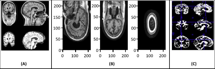
The raw image data require preprocessing, and for that, statistical parametric mapping (SPM) is used. SPM is basically a statistical technique utilized for evaluating cognitive activities documented throughout neuroimaging tests. The statistical parametric mapping software system is additionally used for spatial standardization, smoothing, and statistical analyses of the parametric images. The original magnetic resonance images were initially stripped of the skull and segmented using the segmentation algorithm based on the probability mapping and then standardized using affine registration on the International Brain Mapping Template. The setup comprised bias, noise, and overall intensity calibration. The traditional way of preprocessing would have created image records having 122X145X122 standardized size. The removal of the skull and normalization offered equivalence within the images by simply adjusting the brain's initial image into normal image space and positioning the same brain substructures with the image's coordinates alongside similar images of different participants. Fig. (2) presents the preprocessing of MRI skull images.
4. RESULTS AND DISCUSSION
A CNN (Convnet) is a particular kind of neural network made up of input, several hidden layers, and output layers. The most crucial layer for feature extraction is the hidden layer. It comprises a convolution layer (detects pattern), a rectified linear unit (ReLU) (used to get rectified feature map), a pooling layer (uses filters to detect edges, etc.), and a fully connected layer. Another main advantage of ConvNet is that it assumes that the input data is image only, which helps to embed certain properties into it.
4.1. AlexNet
In this research, AlexNet architecture has been used as a CNN classifier. AlexNet is a popular and precise CNN architecture that has made its name in machine learning and AI, notably in image processing. The basic advantage of this architecture is that it has a pooling layer after every convolutional layer, and we can modify the convolution layer as it does not have a fixed size, which gives us more control over the CNN. It consists of 11X11, 5X5, and 3X3 convolutions, max pooling, dropout, data increase, activation of ReLU, and dynamic SGD. After each convolutional and fully connected layer, ReLU activations are attached.
We looked at two different architectures, AlexNet and GoogleNet, because they have been found to be successful for similar issues [10, 11]. AlexNet was at par with GoogleNet. In both of the trained architectures, 25000 random images of the test dataset were used to compare the accuracy of the two architectures. Then the confusion matrices and the accuracy for each test dataset were calculated for both the architectures.
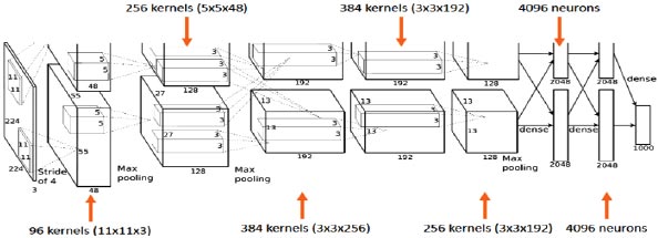
AlexNet's input is a 224x224x3 RGB image that passes through the first convolution layer with 96 feature maps or filters with a size of 11X11 and a 4 stride. The image is now 55x55x96 in size. The AlexNet then performs a maximum layer of pooling or sub-sampling using a 3 subterranean filter and a 2-step process. The final image will be smaller, measuring 27x27x96 in dimensions. The primary variation in our AlexNet versus the standard AlexNet comes in the second layer. The second convolution layer receives data coming from the first convolution layer, and then screens it with 256 feature maps of dimension 5X5X64. Subsequently, the next convolution layer is connected to the data coming from the second convolution layer by 384 feature maps of dimension 3X33X192. The next layer of convolution has 384 feature maps of dimension 3X3X84, and the fifth layer of convolution has 256 feature maps of dimension 3X3X56, as shown in Fig. (3). These are the ideal dimensions for feature extraction purposes in these types of images to train them properly. In the sixth layer, the output is flattened through a fully connected layer in order to accommodate all the data coming from AlexNet architecture; in our system, we have done some minute adjustments, i.e., a fully connected layer is included with 985 neurons in the base model with a softmax layer to deal with negative loss.
4.2. Activation Function
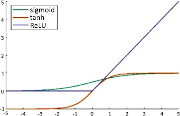
An artificial neuron's activation function is the part of the neuron that produces an output in response to inputs. In AlexNet, ReLU is used as an activation function instead of Tanh and sigmoid. The ReLU activation function is used to add non–linearity and different activation functions, as shown in Fig. (4).
The hyperbolic tangent function is defined in Eq. (1):
 |
(1) |
The sigmoid function is defined in Eq. (2):
 |
(2) |
These functions are slow to train. Because the ReLU does not activate all the neurons at once, it has an advantage over other activation mechanisms. It means that in the ReLU operation, if the input is negative, it converts it to zero and, therefore, the neuron does not get activated. Rectified linear unit (ReLU) is faster to train, and can be done using Eq. (3):
 |
(3) |
It enhances the training speed at the same accuracy by 6 times.
4.3. Fine-tuning
The optimizer we tended to use was the Adam optimizer; one of the algorithms that work well across a wide variety of deep learning architectures is the adaptive moment estimation or Adam optimization algorithm. Adaptive moment estimate (Adam) [14] calculates for each parameter the adaptive learning rates. It is also referred to as a solver. The falling averages of the past and past square gradients, mt and vt, can be calculated using Eqs. (4 and 5):
 |
(4) |
 |
(5) |
The method's names, mt and vt, represent estimates of the gradients' first moment (the mean) and second moment (the uncentered variance), respectively. They balance out these biases by computing bias-correction, first, and second moment estimates using Eqs. (6 and 7):
 |
(6) |
 |
(7) |
We used these to update the parameters in order to give the update rule for Adam, as presented in Eq. (8):
 |
(8) |
4.4. Fine-tuning of the Linear Fully-connected Layer
As we know that the network's end layers tend to be much more precise to the class features in the initial dataset and that the pretrained AlexNet dataset varies from the initial dataset, to tackle this situation, we have to replace the last classifying layer and also calibrate all the classifiers. To solve this problem, first, the fully connected layer is back propagated and its weights are kept in the earlier convolution layer.
The final layer of convolution and the classifiers formulated are calibrated on the observation that the network’s end layer contains more precise characteristics for the dataset. We, however, cannot discover that only calibrating it for the fully connected layer will solve all the problems. Subsequently, we have carried out some trials to adjust the final output layer by the use of the last convolution layer. Mainly because contorting the initial parameters can be disastrous for the network, in our research, the learning rate or we can say the weight-controlling parameter that we have used was 1e−4; the learning rate was increased for enhanced learning and fine-tuning, which showed better performance than the standard learning rate.
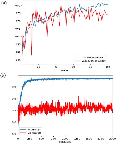
In our experiment, with learning rate 1e-3, the max validation accuracy achieved was 80% and the max training accuracy was 85%, as shown in Fig. (5a), and when we increased the learning rate to 1e-4, we achieved max validation accuracy as 82% with corresponding training accuracy as 96.5%, as shown in Fig. (5b).
Additionally, as mentioned earlier, the improper initialization of the network parameter could impact the performance of the network. But to set the initial parameter uniformly, there are various algorithms available, and we have used the Xavier initialization algorithm based on some research. Support vector machine (SVM) was used for the final classification and AlexNet as an extractor.
4.5. Transfer Learning
A small dataset limits the use of a complex neural network as it would overfit the training data, while transferring learning shows good performance by using a pre-trained network (e.g., AlexNet) to extract features or fine-tune parameters. After finishing AlexNet's higher layer, we achieved 86 percent accuracy in the AD/normal classification. We ensured that the weights were not too small as well as not too large to accurately propagate the signals. Initialization is important for a small network with a limited number of layers; thus, a significant variance can be there while initializing the weights for distribution having zero mean and variance using Eq. (9):
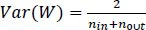 |
(9) |
Where, nin and nout are, respectively, the numbers of inputs and outputs in the layer.
4.6. Evaluation Metrics
For the evaluation metrics, the F1 score, accuracy, precision, recall, and false negative scores are used, in addition to the confusion matrix. True positive and true negative values are stored in a form that resembles a table in a confusion matrix. There are four parts to it; in the first scenario, also known as true positive (TP), the data are verified to be accurate. The second type is a false positive (FP), which involves the values that have been found to be false but are actually true. False negatives (FN) constitute the third category, in which the value actually being positive is found. The fourth one, true negative (TN), genuinely determines the negative value.
Eq. (10) defines accuracy as the proportion of cases that meet the criteria for the dataset divided by the total number of occurrences.
 |
(10) |
Precision is defined as the average likelihood of obtaining pertinent data in Eq. (11).
 |
(11) |
Recall is defined as the typical condition likelihood of full recovery and is represented by Eq. (12).
 |
(12) |
After determining the precision and recall of the classification problem, the F-measure was calculated by combining the two scores. The traditional F-measure computation is shown in Eq. (13).
 |
(13) |
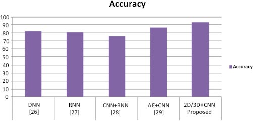
To perform classification using SVM, we performed the experiment using different layers of output features. Previous studies [11-13] have suggested that generic characteristics are usually extracted from lower layers. Our results have indicated that these generic features are not good for SVM classification (the accuracy is 55%), while the features in the higher layers contain more specific characters that can be distinguished by a linear SVM (the accuracy is 85%). Table 1 presents performance parameter values for different datasets. Table 2 compares the suggested method with current methods in a comparative analysis. Our method has yielded superior outcomes to those already achieved. The effectiveness of the proposed model has also been compared to current models, as shown in Table 2, and the suggested model has outperformed the existing models in terms of accuracy. Table 2 illustrates how our model's accuracy compares to that of the models proposed earlier [25-28] at 82.22%, 81%, 74% and 86.47%, respectively. Fig. (6) displays the graphical comparison of the proposed method with state-of-the-art methods.
We have presented two basic CNN architecture models, 2D-CNN and 3D-CNN, for the application of multi-class and binary medical image classification algorithms. These models have been assessed based on the accuracy measure by contrasting their performance to other cutting-edge models, as indicated in Table 1, and a comparison of the proposed work with state-of-the-art methods is tabulated in Table 2.
| Datasets | 2D CNN | 3D CNN | ||||
|---|---|---|---|---|---|---|
| Precision | Recall | F1 score | Precision | Recall | F1 score | |
| AD | 00.95 | 00.92 | 00.94 | 00.97 | 00.93 | 00.95 |
| ADNI | 00.94 | 00.91 | 00.92 | 00.95 | 00.91 | 00.93 |
| NC | 00.97 | 00.93 | 00.96 | 00.93 | 00.95 | 00.94 |
| Methods | Datasets | Techniques | Performance |
|---|---|---|---|
| [25] | Gene expression and DNA methylation profiles |
DNN | Accuracy (NC/AD): 82.3% |
| [26] | Demographic information, neuro-imaging |
RNN | Accuracy (CN/MCI/AD): 81% |
| [27] | MRI | CNN + RNN | Accuracy (NC/AD): 91.0% Accuracy (NC/MCI): 75.8% Accuracy (sMCI/pMCI): 74.6% |
| [28] | MRI | AE+ CNN | Accuracy (AD/NC): 86.60% |
| Proposed | ADNI | 2D/3D CNN | Accuracy: 93.24% |
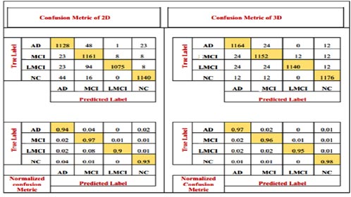
The number of patients diagnosed with NC and AD and the number of patients diagnosed with MCI are all depicted in the confusion matrix. It shows the number of patients diagnosed as MCI as well as others. The model has also been accompanied by the numerical, reciprocal, and normalized confusion matrices, as depicted in Fig. (7).
CONCLUSION
The proposed work aimed to classify Alzheimer's disease (AD) using transfer learning methods. We used strict pre-processing steps on raw MRI data from the ADNI dataset and used the AlexNet, i.e., CNN classifier on pre-processed data to classify Alzheimer’s disease. During classification, features of low to high levels were learned. We increased the learning rate to enhance the prediction of our model. For future classification of neural networks, pre-trained convolution layers capable of extracting generic image features, such as pre-trained AlexNet convolution layers on CNN, could provide good input features. These findings suggest that deep neural networks may be capable of autonomously learning as to which imaging indicators are suggestive of Alzheimer's disease and using them for accurate early disease detection. The proposed techniques have been found to possess a 93.24% accuracy rate. Deep learning-based AD research is still under development for improved performance and transparency. Resources for heterogeneous neuroimaging data and computation are expanding quickly. Despite the need for approaches to combine various forms of data in a deep learning network, research on the diagnostic categorization of AD using deep learning is moving away from hybrid methods and towards a model that uses just deep learning algorithms.
LIST OF ABBREVIATIONS
| AD | = Alzheimer's disease |
| MRI | = Magnetic resonance imaging |
| CNN | = Convolutional neural network |
| MCI | = Moderate cognitive impairment |
| ADNI | = Alzheimer's disease neuroimaging initiative |
| NC | = Normal control |
| SVM | = Support vector machine |
ETHICS APPROVAL AND CONSENT TO PARTICIPATE
Not applicable.
HUMAN AND ANIMAL RIGHTS
No humans/animals were used for studies that are the basis of this research.
CONSENT FOR PUBLICATION
Not applicable.
AVAILABILITY OF DATA AND MATERIALS
The data and supportive information are available within the article.
FUNDING
None.
CONFLICT OF INTEREST
Dr. Vinayakumar Ravi is the associate editorial board member of the journal The Open Bioinformatics Journal.
ACKNOWLEDGEMENTS
Declared none.